What does Maple do when you ask it to display a solution of a differential equation with DEplot? Obviously, it cannot solve the equations analytically, since solutions don't always exist in closed form. Instead, it approximates them numerically.
More precisely, given a differential equation and an initial condition
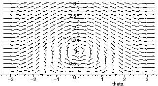
Maple doesn't typically use Euler's method because the errors accumulate too quickly. To see this, we reproduce one of the earlier figures from §2 using Euler's method.
>
  DEplot( phug, [theta(t), v(t)], t=0..5,
      [seq([theta(0)=0, v(0)=1+0.2*i], i=0..10)],
      theta=-Pi..3*Pi, v=0.01..3, linecolor=black, method=classical[foreuler]);
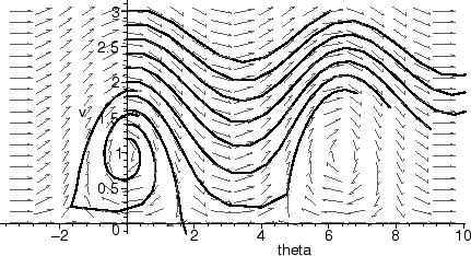
While the errors in the above figures are considerable, using a much smaller stepsize (say, stepsize=0.01) will essentially reproduce the earlier figure, with a lot more computation.
To get some ideas about improving on Euler's method, let's first notice that Euler's method corresponds exactly to the left-hand Riemann sum when computing a numerical approximation to an integral. You may recall from calculus that the left-hand sum converges to the value of the integral, but you must take a large number of subdivisions to get any accuracy.
A more efficient method is the trapezoid rule, which is the average of the
left-hand and right-hand sum. There is a numerical scheme for integrating
ODEs which corresponds to this, known variously as the improved Euler
method or the Heun formula. In the trapezoid rule, we compute the
function at the left and right endpoints of the function and average the
result; the analog of this would require us to average the value of the
vector field at our current point and at the next point. Perhaps you see
the circularity implicit in that reasoning: to know the next point, we would
need to solve the differential equation. So, instead we fudge a bit: we get
our approximation of the next point by using Euler's method. More
specifically, using the notation of §4.1, given an
approximation ![]() at time ti, we find the next one using the
scheme below.
at time ti, we find the next one using the
scheme below.
| ti + 1 | = | ti + h | ||
| = | slope at the left side of the interval | |||
| = | slope at the right side of the interval | |||
| = | xi + h( |
To do the improved Euler method, we need to evaluate the vector field twice as often as the regular Euler method, but there is a big gain in accuracy. The error of the approximation for a fixed time interval is proportional to h2. Thus, if we decrease h by a factor of 10, we should expect to reduce the error 100-fold. You can get Maple to use the improved Euler method by specifying method=classical[heunform] as an argument to DEplot and related commands.
You might remember from your calculus course that Simpson's rule can get
very accurate numerical approximations for integrals with a very few number
of points. This is because Simpson's rule is a fourth-order method: the
error in the approximation is proportional to h4. For Simpson's rule, we
evaluate the function at the right endpoint, the left endpoint, and the
middle, and then take a weighted average of those values.
The analog of Simpson's rule for differential equations is called the Runge-Kutta method3.2, developed by the German mathematicians C. Runge and W. Kutta at the end of the nineteenth century. It takes a linear combination of four slopes, as below:
| ti + 1 | = | ti + h | ||
| = | slope at the left side of the interval | |||
| = | slope at the middle of the interval | |||
| = | corrected slope at the middle of the interval | |||
| = | slope at the right side of the interval | |||
| = | xi + h( |
Runge-Kutta is probably the most commonly used method of numerical integration, because of its generally high accuracy. Like Simpson's rule, it is a fourth-order method, so the error is proportional to h4. Maple has several numerical methods for ODEs built in to it; see the help page on dsolve[numeric] for more information about them; the ones we have described are ``classical'' methods, and are described (along with others) on Maple's help page for dsolve[classical]. Unless asked to do otherwise, Maple's DEplot command uses the fourth-order Runge-Kutta method described above (Maple's name for this method is classical[rk4]), although the numeric option of dsolve defaults to a variation called fourth-fifth order Runge-Kutta-Fehlberg, which Maple refers to as rkf45.