
Now that we have some equations in hand, our first goal is to understand what the solutions look like. Note that the equations are nonlinear, and we cannot hope to find explicit formulae for the solutions-- they don't exist except in very special cases.
Let's deal with the easiest case first: pretend that drag doesn't exist and set R = 0. Does this help?
The equations become

Now, let's see what we can say about the solutions to this equation. First, notice that there must be many solutions: Any choice of initial conditions
There is one very easy solution to find.
Notice that if we can find a choice of ![]() and v so that
and v so that
![]() = 0 =
= 0 = ![]() , then since their derivatives are zero,
v(t) and
, then since their derivatives are zero,
v(t) and ![]() (t) must be constant functions. But solving this is
simple:
(t) must be constant functions. But solving this is
simple:

What about other solutions? Now we must work harder. There is no hope to find a general analytic expression for v(t) and
First, notice that such a solution ![]() can be thought of as a
parametric curve in the
(
can be thought of as a
parametric curve in the
(![]() , v)-plane which passes through the point
, v)-plane which passes through the point
![]() (0) = [
(0) = [![]() , v0]. At any point along this parametric curve,
we can calculate its derivative:
, v0]. At any point along this parametric curve,
we can calculate its derivative:
We can get an idea of how the solutions behave by making a picture of the
vector field corresponding to this: At each value for the pair
(![]() , v), we draw the vector
, v), we draw the vector
![]()
![]() ,
,![]()
![]() , which only
depends on
(
, which only
depends on
(![]() , v).
, v).
To get maple to do this, we can use the fieldplot command. Because the arrows in the fieldplot show not only direction but also relative magnitude, we shouldn't get too close to the v = 0 axis or they will overwhelm the smaller arrows for which occur for larger v.
>
  plots[fieldplot]( [ (v^2 - cos(theta))/v, -sin(theta) ],
                    theta=-Pi..Pi, v=0.2..3, arrows=slim);
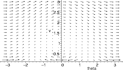
We can certainly see that near the constant solution
{![]() = 0, v = 1},
nearby solutions rotate around it in a clockwise manner. This ``rotation''
in the
= 0, v = 1},
nearby solutions rotate around it in a clockwise manner. This ``rotation''
in the ![]() - v coordinates corresponds to a flight path which wobbles:
the nose angle alternately increases and decreases, as does the
velocity. For v large, it seems that the solutions move from left to
right--
- v coordinates corresponds to a flight path which wobbles:
the nose angle alternately increases and decreases, as does the
velocity. For v large, it seems that the solutions move from left to
right-- ![]() constantly increases, which means that the glider is
always increasing its nose angle. This means it is doing loops.
constantly increases, which means that the glider is
always increasing its nose angle. This means it is doing loops.
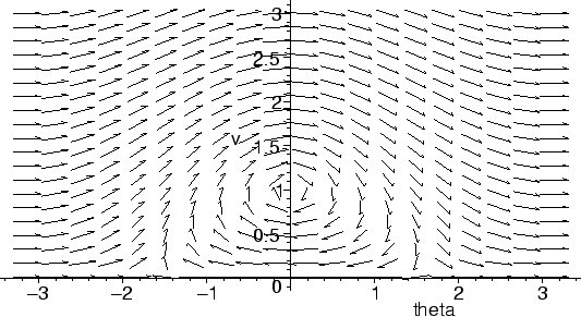
We can also use the DEplot command from Maple's DEtools
package to produce a direction field. The direction field is obtained from
the vector field by rescaling all nonzero vectors to be of unit
length. Sometimes discarding the extra information makes it easier to see
what is happening. In addition, DEplot has other very useful
options, and will be one of our primary tools throughout this chapter.
For convenience, we will name our system of differential equations as
phug, so that we needn't keep retyping them.
>
  phug := [ diff(theta(t),t) =  (v(t)^2 - cos(theta(t)))/v(t),
            diff(v(t),t)     =  -sin(theta(t)) - R*v(t)^2 ];
  R:=0;
![\begin{maplelatex}
\begin{displaymath}
\mathit{phug} := [{\frac {\partial }{\par...
...)]
\end{displaymath}\begin{displaymath}
R := 0
\end{displaymath}\end{maplelatex}](img274.gif)
>
  with(DEtools):
  DEplot( phug, [theta(t), v(t)], t=0..1, theta=-Pi..Pi, v=0.01..3);
We can also ask maple to plot a number of solutions corresponding to several initial conditions. Rather than typing in 11 initial conditions, we can use seq to generate them. We tell maple that the solution curves should be black, because otherwise it uses a sickly yellow. If we had wanted each solution curve to be a different color, we could use something like linecolor=[seq(COLOR(HUE,i/10),i=0..10)].
>
  DEplot( phug, [theta(t), v(t)], t=0..5,
          [seq([theta(0)=0, v(0)=1+0.2*i], i=0..10)],
          theta=-Pi..3*Pi, v=0.01..3, linecolor=black );
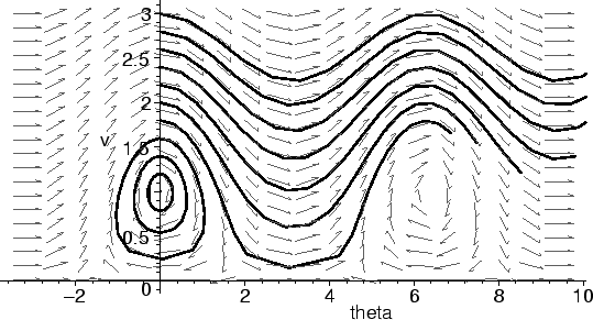
The above figure confirms our earlier impressions about the ``wobbling'' and ``looping'' solutions. We'll see how to get Maple to demonstrate this more explicitly in section 5, where we will plot the path of the glider through space (i.e., in x-y coordinates).
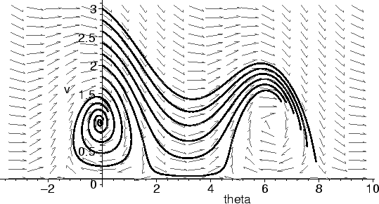
Just to see how things differ if we make R nonzero, let's change R and
get Maple to show us what happens. We need to adjust the stepsize to get a
reasonable accuracy; what precisely this does is described in the next
section.
>
  R:=0.1;
  DEplot( phug, [theta(t), v(t)], t=0..5,
          [seq([theta(0)=0, v(0)=1+0.2*i], i=0..10)],
          theta=-Pi..3*Pi, v=0.01..3, linecolor=black, stepsize=0.1 );
>
  R:=3;
  DEplot( phug, [theta(t), v(t)], t=0..5,
          [seq([theta(0)=0, v(0)=1+0.2*i], i=0..10)],
          theta=-Pi..3*Pi, v=0.01..3, linecolor=black,stepsize=0.1 );
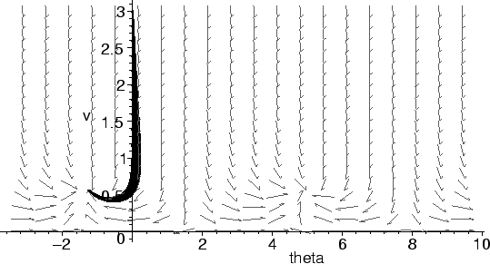
The behavior of the glider appears to be dramatically affected by the drag parameter R. One of our main goals in this chapter will be to classify the types of solutions that are possible as a function of the drag parameter R.