Next: Dealing with the Singularity
Up: The Art of Phugoid
Previous: Fixed Point Analysis
This analysis of the previous section allows us to completely classify what
happens in the Phugoid model for all
R  [0,
[0, ). In all cases, the
fixed point in
(
). In all cases, the
fixed point in
( , v) coordinates corresponds to the solution

(
t) = - arctan
 R
R
 v
v(
t) =
![$\displaystyle \sqrt[4]{\frac{1}{1 + R^2}}$](img351.gif) x
x(
t) =
 y
y(
t) =

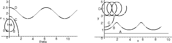
- R = 0:
- In this case, there is no drag. The fixed point at
= 0, v = 1
corresponds to a glider flying level with a constant speed (labeled A
in the figures below). The fixed point is a center in , v
coordinates: nearby solutions are closed curves and correspond to a glider
with an oscillatory path, alternately diving and climbing (labeled B).
For initial conditions further away from the fixed point, v(t) oscillates,
but (t) constantly increases (see D). Such solutions correspond
to a glider endlessly looping, and a pilot with a severe case of nausea.
Between these two is a solution which cannot be continued beyond a certain
time (C), because v(t) becomes zero and our equations are no longer
defined. This corresponds to a glider which stalls.
-
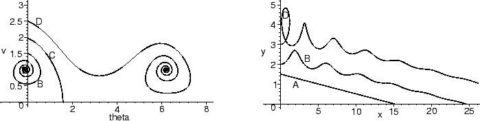
0 < R < 2
 :
:
- Here the fixed point (A) corresponds to a glider which dives
with a constant velocity and not too steep an angle (the steepest angle is
slightly less than
 /4 below horizontal). The fixed point is a spiral
sink: nearby initial conditions spiral into it (B). Such a spirals
corresponds to a glider for which the angle and velocity constantly
oscillate, but these oscillations get smaller and smaller as time passes,
limiting on the same angle and velocity as the fixed point. Solutions with
initial conditions further away (D) from the fixed point do some
number of loops before settling into a pattern of oscillations which limit
on the diving solution. Between the solutions which do k loops and those
which do k + 1 loops lies a solution which stalls out after k
loops (C) -- at some time the solution gets to
= 2k + /2
(i.e. going straight up) and velocity v = 0.
/4 below horizontal). The fixed point is a spiral
sink: nearby initial conditions spiral into it (B). Such a spirals
corresponds to a glider for which the angle and velocity constantly
oscillate, but these oscillations get smaller and smaller as time passes,
limiting on the same angle and velocity as the fixed point. Solutions with
initial conditions further away (D) from the fixed point do some
number of loops before settling into a pattern of oscillations which limit
on the diving solution. Between the solutions which do k loops and those
which do k + 1 loops lies a solution which stalls out after k
loops (C) -- at some time the solution gets to
= 2k + /2
(i.e. going straight up) and velocity v = 0.
-
R
 2:
2:
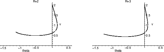
- The fixed point is a sink corresponding to a steeply diving
solution.3.6Causing the glider to loop becomes increasingly difficult as R
increases. For example when R = 3, if the initial angle is
zero, an initial velocity of larger than 86.3 is required to get the
glider to do one loop. If the initial angle differs from that of the
fixed point, the glider fairly quickly turns towards that angle. No
oscillation occurs; the angle can pass the limiting angle at most once.
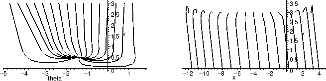
We have shown that for
R < 2, the fixed point is a spiral
sink: nearby solutions oscillate toward it. We should, however, point
out that while the oscillations are always present mathematically,
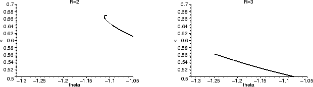
they can be very hard to discern. To emphasize this, we will compare
a solution in the , v-plane for R = 2 (a spiral sink) and R = 3
(a sink with two real eigenvalues).
The two plots look rather similar. However, if we look closely at the
solutions near the fixed point (we can use zoom to do this
without recomputing the picture), we see a significant difference.
For R = 2, there is a ``hook'' at the end, but for R = 3, the solution
goes straight in to the fixed point. Further magnifications show the
same pattern, as you may want to verify for yourself. The spiral for
R = 2 is always present, but very tight and hard to detect.
Similarly, the oscillations in the x, y-plane when R is just
slightly less than 2 are nearly indiscernable, but present.
Footnotes
- ...
solution.3.6
-
For
R = 2, the linearization corresponds to a degenerate case
with a double eigenvalue, rather than a regular sink. However, what
we say here still applies.
Next: Dealing with the Singularity
Up: The Art of Phugoid
Previous: Fixed Point Analysis
Translated from LaTeX by Scott Sutherland
2002-08-29