
Celestial Mechanics on a Graphing Calculator
An analytic treatment of the Two-body problem is in Eric Weisstein's Treasure Trove
of Physics.
Marshal Hampton at the University of Washington has a page on
Central
configurations in the n-body problem with a lovely animation of
a configuration studied by Lagrange. The
Astronomy Workshop at the University of Maryland has a nice page
on Orbital Simulations (but their Satellite Viewer crashed my Netscape).
DIFFERENTIAL
EQUATIONS AND OSCILLATIONS is a web resource by Rubin H. Landau of
Oregon State University, with a description of Euler's Method and
the Runge-Kutta Algorithm. Comparison of the efficiency of the
algorithms is treated on G. Bard Ermentrout's Numerical Methods page at Carnegie
Mellon (useful although some links are dead).
1. Newton's laws
Isaac Newton laid down the law in outer space.
The vast majority of motion in space is governed by two laws,
both first propounded by him (Principia, 1687).
- The Law of Motion. A body in space travels in a constant
direction at constant speed unless a force acts on it. And then
the velocity vector changes (the body accelerates) according to
the force. More specifically, if the
body has mass m, and
velocity v, and is acted upon by a force F,
then
An informal way to understand this equation is to think that,
if the body is traveling with velocity v
at time t,
then at an infinitesimally later time t + dt its velocity
will be v + (F/m)dt.
By that time its position will have changed by vdt.
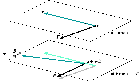 Acceleration in space.
The body is traveling with velocity v
at time t;
at time t + dt its velocity
will be v + (F/m)dt.
By that time its position will have changed by vdt.
At time t + dt the body feels the force vector corresponding
to its new position, and the story recycles. (This image does not make
complete sense because it is impossible to draw infinitesimal
vectors. When the dts are sent back to the denominators
everything has meaning, but the picture evaporates.)
Acceleration in space.
The body is traveling with velocity v
at time t;
at time t + dt its velocity
will be v + (F/m)dt.
By that time its position will have changed by vdt.
At time t + dt the body feels the force vector corresponding
to its new position, and the story recycles. (This image does not make
complete sense because it is impossible to draw infinitesimal
vectors. When the dts are sent back to the denominators
everything has meaning, but the picture evaporates.)
- The Law of Gravitation. Gravity attracts masses one
to the other. In order to keep things simple we will not worry about
the shape or composition of the bodies, and will consider only
point masses. Suppose we have a mass m at
position x and a mass m' at
position x'. For future reference, their
distance is d=|x'-x|.
The force of gravitation pulls them towards their common center of mass
at x0 = [mx+m'x']/(m + m'). Acting on m it has has direction x' - x
(points from x to x'). Its
magnitude is Gmm'/d2, G times the
product of the two masses divided by the
square of their distance. The constant G
is universal and depends only on the units chosen.
To write the gravitational force acting on m
as a vector, we take a unit vector pointing
from x to x' : x'-x/d,
and multiply it by the magnitude we have specified:
           Gmm'(x'-x)
    F  =  -----------
              d3
|
- Putting it all together. If we have several bodies
traveling through space, the gravitational force acting on each
one is the vector sum of the attractive force it feels from each
of the others. If we know the initial positions, masses and velocities,
Newton's two laws completely determine the behavior of the system.
What we would like to get is a set of explicit formulas
allowing us to calculate where each body will be at any future instant
in time. In
general, such formulas do not exist. The differential equation
assembled from Newton's two laws cannot be solved explicitly.
- Numerical integration. How do we predict the motions
of the satellites we send through the solar system? We go back to
the infinitesimal scheme shown in the first image. If dt
is replaced by a finite time increment Delta t, then
the expressions vDelta t and
(F/m)Delta t
give approximate
values for the change in position and velocity during the
time interval Delta t. We can calculate the new, approximate,
position and velocity and apply the same procedure to approximate
the total change after 2Delta t, and we can do this over
and over until we get to the time we are interested in.
Obviously, there is a lot of approximation going on; how can
we tell if our predictions are accurate at all? As Delta t
--> 0, the theory guarantees that the error will also go to
zero, but will it do so fast enough for the computation to be
carried out in a reasonable amount of time?
- The restricted 2-body problem is a special case
which can be solved explicitly. Suppose there are just
two bodies, one of which has
negligeable mass compared to the other. For example, a man-made satellite
of mass perhaps 100 tons=105 kg and
the Earth (mass=6x1024 kg); or the
Earth and the Sun (mass=2x1030 kg). In this case, unless
the smaller body has enough velocity to escape
completely, it will travel forever in
an elliptical orbit about the larger.
In this column we will
investigate numerical integration in the restricted 2-body problem.
The approximation
algorithms are simple enough to be run on a graphing
calculator. Readers are urged to experiment on
their own with the programs.
The relative slowness of calculators will
make algorithm efficiency a crucial consideration.
And our knowledge that
after a ``year'' the smaller planet must return to exactly where
it started will give us a simple test of
algorithm reliability.
Tony Phillips
Stony Brook
Comments: webmaster@ams.org
@ Copyright 2001, American Mathematical Society.