Recursion and making a Koch Snowflake with Maple

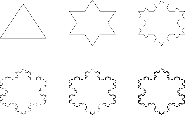
In the previous section, we didn't give the specifics of exactly how we generated the Koch curve of level 5 which we showed. The general procedure was pointed out (``Begin with F. Replace each F with FLFRRFLF. Repeat 5 times.''), but if you actually tried to do it yourself, you might have found it a bit tricky. Since the turtle command for the curve has 2388 letters, certainly it isn't something you would expect someone to type in directly.

Instead, a small maple procedure was written to generate it. Before giving the details, let's analyze the process a bit. We shall rely heavily on the self-similar nature of the Koch curve $\mbox{$\mathcal{{K}}$}$_$\infty$.

Notice that the curve $\mbox{$\mathcal{{K}}$}$_$\infty$ is made up of four small copies of itself, arranged as

$$\mbox{$\mathcal{{K}}$}$$_$\infty$L  $$\mbox{$\mathcal{{K}}$}$$_$\infty$RR  $$\mbox{$\mathcal{{K}}$}$$_$\infty$L  $$\mbox{$\mathcal{{K}}$}$$_$\infty$.

If we use K_n to denote the set of turtle commands used to produce $\mbox{$\mathcal{{K}}$}$_n, then a similar statement is true for each K_n, namely  

K_n = $$\left\{\vphantom{ \begin{array}{ll} K_{n-1}{\mbox{L}} K_{n-1} {\... ...& {\mbox{if}}~ n>0 \\ {\mbox{F}} & {\mbox{if}}~ n=0 \\ \end{array} }\right.$$$$\begin{array}{ll} K_{n-1}{\mbox{L}} K_{n-1} {\mbox{RR}} K_{n-1}{... ..._{n-1} & {\mbox{if}}~ n>0 \\ {\mbox{F}} & {\mbox{if}}~ n=0 \\ \end{array}$$ $$\left.\vphantom{ \begin{array}{ll} K_{n-1}{\mbox{L}} K_{n-1} {\m... ...& {\mbox{if}}~ n>0 \\ {\mbox{F}} & {\mbox{if}}~ n=0 \\ \end{array} }\right.$$.

Recursive functions.

This is an example of a recursive definition. You've probably encountered such definitions previously in math classes. For example, the factorial function can be defined either as

n! = n ^. (n - 1) ^. (n - 2) ^... 3 ^. 2 ^. 1

or

n! = $$\left\{\vphantom{ \begin{array}{ll} n\cdot (n-1)! & {\mbox{if}}~ n>1 \\ 1 & {\mbox{if}}~ n=1 \\ \end{array} }\right.$$$$\begin{array}{ll} n\cdot (n-1)! & {\mbox{if}}~ n>1 \\ 1 & {\mbox{if}}~ n=1 \\ \end{array}$$ $$\left.\vphantom{ \begin{array}{ll} n\cdot (n-1)! & {\mbox{if}}~ n>1 \\ 1 & {\mbox{if}}~ n=1 \\ \end{array} }\right.$$.

The second definition is much simpler to implement in a programming language which allows recursive functions, such as maple.^4.5 To see this, let's implement the factorial function in both ways:

> fact1 := proc(n::posint)
    local i,ans;
    ans := 1;
    for i from 1 to n do
      ans := ans*i;
    od;
    ans;
  end:

> fact2 := proc(n::posint)
    if (n=1) then
        1;
    else
       n*fact2(n-1);
    fi;
  end:

Notice how much shorter and clearer the second version is.^4.6 However, there is a price to pay: a recursively defined function has a bit more overhead than a non-recursive one. However, the savings in simplicity often overwhelms the minor loss in speed.^4.7

To test your understanding, you might try to write a procedure to generate the Fibonacci numbers, which are defined by

F(n) = $$\left\{\vphantom{ \begin{array}{ll} F(n-1) + F(n-2) & {\mbox{if}}~n > 2 \\ 1 & {\mbox{if}}~n=1~{\mbox{or}}~n=2\\ \end{array} }\right.$$$$\begin{array}{ll} F(n-1) + F(n-2) & {\mbox{if}}~n > 2 \\ 1 & {\mbox{if}}~n=1~{\mbox{or}}~n=2\\ \end{array}$$ $$\left.\vphantom{ \begin{array}{ll} F(n-1) + F(n-2) & {\mbox{if}}~n > 2 \\ 1 & {\mbox{if}}~n=1~{\mbox{or}}~n=2\\ \end{array} }\right.$$.

Try to implement this with both a recursive and non-recursive procedure. The non-recursive one is much more complicated!

A recursive procedure to generate K_n

With the idea of recursion in our bag of tools, we can now easily write our procedure to generate the Koch curve, using the observation we made in §3, namely that

K_n = $$\left\{\vphantom{ \begin{array}{ll} K_{n-1}{\mbox{L}} K_{n-1} {\... ...& {\mbox{if}}~ n>0 \\ {\mbox{F}} & {\mbox{if}}~ n=0 \\ \end{array} }\right.$$$$\begin{array}{ll} K_{n-1}{\mbox{L}} K_{n-1} {\mbox{RR}} K_{n-1}{... ..._{n-1} & {\mbox{if}}~ n>0 \\ {\mbox{F}} & {\mbox{if}}~ n=0 \\ \end{array}$$ $$\left.\vphantom{ \begin{array}{ll} K_{n-1}{\mbox{L}} K_{n-1} {\m... ...& {\mbox{if}}~ n>0 \\ {\mbox{F}} & {\mbox{if}}~ n=0 \\ \end{array} }\right.$$.

> Koch:= proc (n::nonnegint)
    if (n=0) then
       `F`;
    else 
        cat( Koch(n-1), `L`, Koch(n-1), `RR`, Koch(n-1), `L`, Koch(n-1));
    fi;
  end:

> Koch(2);

If you think about it for a second, you might notice that what we have just done is to write a little program (Koch) whose output is a program in another language (the string of turtle commands which describe K_n). While this may seem odd at first, doing this sort of thing is not at all uncommon.

The Koch Snowflake

Often, one sees the curve $\mbox{$\mathcal{{K}}$}$_$\infty$ as one side of a closed plane figure, the Koch Snowflake (sometimes also called the ``Koch Island''). This is an infinite length ``curve'' which bounds a finite area, and resembles a snowflake. It is made by sticking together three copies of $\mbox{$\mathcal{{K}}$}$_$\infty$ meeting each other at 60 degrees angles so that they close up. We do this now:

> KochFlake := proc(n::nonnegint)
   ResetTurtle();
   SetTurtleAngle(60);
   cat(`L`,Koch(n),`RR`,Koch(n),`RR`,Koch(n));
  end:

> plots[display](array([[seq(TurtleCmd(KochFlake(i)),i=0..2)],
                        [seq(TurtleCmd(KochFlake(i)),i=3..5)]]));

Some variations on the Koch curve

What happens to the curve $\mbox{$\mathcal{{K}}$}$_$\infty$ if we change the height of the bumps we add at each stage? We can do this easily by changing the angle the turtle turns when it encounters an R or an L. For example, an angle of 10 degrees gives a curve which is nearly smooth.

> ResetTurtle(); SetTurtleAngle(10);
  TurtleCmd(Koch(6));

But an angle of 80 degrees gives a curve which wiggles wildly and almost seems to take up area.

> ResetTurtle(); SetTurtleAngle(80);
  TurtleCmd(Koch(6));

We shall make this observation more precise in section 5. You might try some additional experiments on your own, to gain intuition about how the limit curve depends on the parameters. For example, what would happen if you make the angle be 90 degrees? Do you find the result surprising?

Some other variations you might want to try on your own might be to modify the Koch procedure so that the bumps are added alternately above and below the curve, as shown in the following figure:

Here the angle used was less than 60 degrees. What happens for an angle of exactly 60 degrees? How about a larger angle? Can you adjust things so that using 75 degrees angle does not cause self-intersections?

Or, you might try using a different shape of a bump. For example, below we used squares, shrinking the scale first so the bumps don't run into each other. What happens if you vary the scale factor with SetTurtleScale?

Footnotes

... maple.^4.5

Most programming languages these days do allow recursive function calls, although this was not the case until 1985 or so.

... is.^4.6

We've stretched things a bit here. We could have implemented the factorial even more simply as fact3:=n->product(i,i=1..n);. However, this relies on the fact that the factiorial is a special product.

... speed.^4.7

Also, symbolic systems such as maple often have additional means to speed up recursive procedures. If you expect your function to be called several times with the same argument, you can add options remember to the definition. This instructs maple to save the result of previous function calls. When the function is called again, maple just gives the same result as before, rather than computing it again. But be careful: you get the same answer, even if you change the function later.