shell5

$e-MATH$

The Mathematical Study of Mollusk Shells

5. Mathematical models of helical shells

Once the constants c and v are known, the entire shell can be generated from the knowledge of one cross-section: each point (x,y,z) generates the curve F(t) = e^(vt)(x cos(ct) + y sin(ct), -x sin(ct) + y cos(ct), z), and these curves together generate the entire surface of the shell.

In generating the models for this column, I have assumed that the section is an ellipse in the (x,z)-plane, of the form (h + a cos s, 0, k + b sin s), for s between 0 and 2 Pi. (For more general cross-sections see Randolf Schultz's Shelly page.) The Maple instruction that generates the mathematical models is plot3d([exp(v*t)*(h+a*cos(s))*cos(t),-exp(v*t)*(h+a*cos(s))*sin(t), exp(v*t)*(k+b*sin(s))],s=0..2*Pi,t=-10..-1,grid=[30,50],scaling=constrained); The constants v,a,b,h,k were chosen by eye, without careful measurements, to give the best match to the available images. Their effect on the shape of the shells is shown in the examples below and in the Flat-coil examples (k=0).

v=.05, c=1, a=1, b=1.2, h=1.5, k=-8.5, t=-40..-1

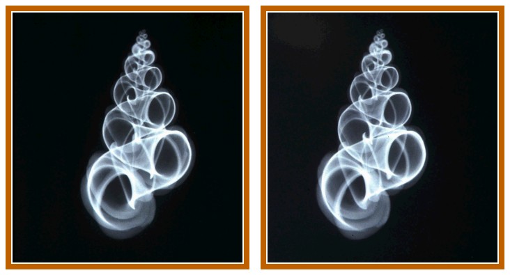
Radiograph of Epitonum scalare. This is half of a stereo pair from Peter Abrahams' page and is used with permission.

Epitonum scalare, the Precious Wentletrap. Image from Sanibel Seashell Industries, used with permission.

v=.075, c=1, a=1.6, b=1.6, h=1.5, k=-7, t=-40..-1

Fossil Pseudoheliceras subcatenatum (an Ammonite). Image @2000 Jim Craig from Fossils of the Gault Clay and Folkestone Beds of Kent, UK, used with permission. Note that this shell coils to the left.

v=.18, c=1, a=2.6, b=2.4, h=1.25, k=-2.8, t=-20..1

Natica stellata, Orange Moon. Image from Sanibel Seashell Industries, used with permission.