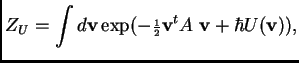
The integrals of interest in Physics have the form
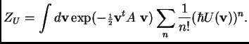
If ![]() is a monomial in the coordinate functions
is a monomial in the coordinate functions
![]() , then each term in the
sum of integrals is a sum of
, then each term in the
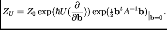
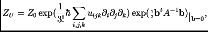
sum of integrals is a sum of ![]() -point functions, and can be evaluated by our method, which can be written symbolically as:
-point functions, and can be evaluated by our method, which can be written symbolically as:
Example: This example is formally like the ``![]() theory.'' We take
theory.'' We take
![]() and analyze
and analyze
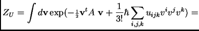
Let us compute the terms of degree 2 in ![]() .
.
These terms will involve 6 derivatives; their sum is:
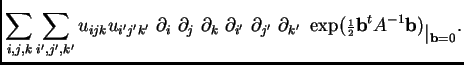
By Wick's Theorem we can rewrite this sum as
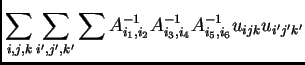
These pairings can also be represented by graphs,
very much in the
same way that we used for ![]() -point functions: there will be one trivalent
vertex
for each
-point functions: there will be one trivalent
vertex
for each ![]() factor, and one edge for each
factor, and one edge for each ![]() . In this case there
will be exactly two distinct graphs, according
as the number of (unprimed, primed) index pairs is 1 or 3.
. In this case there
will be exactly two distinct graphs, according
as the number of (unprimed, primed) index pairs is 1 or 3.
Summing over all possible labellings of these graphs will give some duplication, since each graph has symmetries that make different labellings correspond to the same pairing. The ``dumbbell'' graph has an automorphism (symmetry) group of order eight, whereas the ``theta'' graph has an automorphism group of order twelve.
Keeping this in mind, we may rewrite the coefficient of ![]() as:
as:
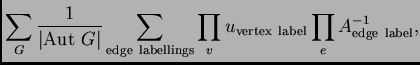
In general, the ``Feynman rules'' for computing the coefficient of
![]() in the expansion of
in the expansion of ![]() are stated in exactly this way,
except that the sum
are stated in exactly this way,
except that the sum ![]() is over trivalent graphs with
is over trivalent graphs with ![]() vertices
(and
vertices
(and ![]() edges).
edges).