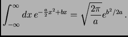
The basic fact from calculus that powers the whole discussion is:
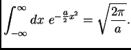
The identity with ![]() is proved by the familiar trick of calculating the square of the
integral in polar coordinates. The general identity follows by change of variable
from
is proved by the familiar trick of calculating the square of the
integral in polar coordinates. The general identity follows by change of variable
from ![]() to
to
![]() .
.
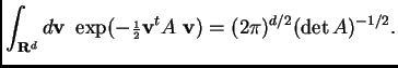
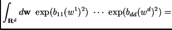
This fact generalizes to higher-dimensional integrals. Set
![]() and
and
![]() , and let
, and let ![]() be a symmetric
be a symmetric ![]() by
by ![]() matrix.
matrix.
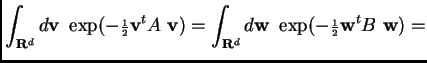
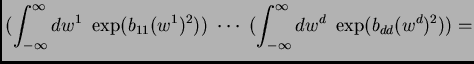
We work the calculation for the case ![]() diagonalizable: in that case there
exists an orthogonal matrix
diagonalizable: in that case there
exists an orthogonal matrix
![]() (so
(so
![]() ) such that
) such that ![]() is the diagonal matrix
is the diagonal matrix ![]() whose only
nonzero entries are
whose only
nonzero entries are
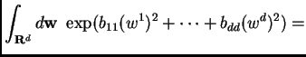
![]() along the diagonal. Then
along the diagonal. Then
![]() and
and
![]() where
where
![]() , using
, using
![]() and
and
![]() . Since
. Since ![]() is orthogonal
is orthogonal ![]() and the change of variable from
and the change of variable from ![]() to
to ![]() does not
change the integral:
does not
change the integral:
The argument in general uses two additional observations: both sides of
the equation vary continuously as functions of the entries in ![]() , and any
matrix
, and any
matrix ![]() with complex coefficients can be approximated to arbitrary
accuracy by diagonalizable matrices.
with complex coefficients can be approximated to arbitrary
accuracy by diagonalizable matrices.
This follows from Proposition 1 by completion of the square in the exponent and a change of variables.
The generalization to ![]() dimensions replaces
dimensions replaces ![]() with
with ![]() as before and
as before and ![]() with
the vector
with
the vector
![]() .
.
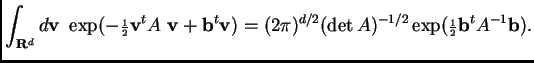
This is proven exactly like Proposition 2.
If we write this integral as ![]() , then the integral of Proposition 2 is
, then the integral of Proposition 2 is ![]() and this proposition can be rewritten as
and this proposition can be rewritten as