Project 2a
Analysis of the case k=0.9
In order to help out a little with project 2a, I present here an analysis of one specific value of the acceleration constant ![]() which exhibits phenomena that we haven't explicitly studied in class. You will need to give a similar analysis for other representative values of
which exhibits phenomena that we haven't explicitly studied in class. You will need to give a similar analysis for other representative values of ![]()
First, we set the stage with our basic definitions.
| > | with(DEtools):
with(plots): with(LinearAlgebra): |
| > | phug:=[ diff(theta(t),t) = (v(t)^2 - cos(theta(t)))/v(t),
diff(v(t),t) = -sin(theta(t)) - 0.4*v(t)^2 + k, diff(x(t),t) = v(t)*cos(theta(t)), diff(y(t),t) = v(t)*sin(theta(t)) ]; |
| (1) |
| > | k:=0.9; |
| (2) |
One important piece of information is where the fixed points are, if there are any. Thus, we solve for which values of ![]() we have
we have ![]() and
and ![]() Since there are some nonphysical solutions (with
Since there are some nonphysical solutions (with ![]() or
or ![]() complex), we exclude those.
complex), we exclude those.
| > | solve( [rhs(phug[1]), rhs(phug[2])=0], [theta(t),v(t)]); |
| (3) |
| > | fix:=subs({theta(t)=theta, v(t)=v},%[1]); |
| (4) |
Above, we plucked out the only meaningful solution, and changed the notation to use θ instead of θ(t), etc.
We need to determine the type of this fixed point (sink, source, etc), which can be done by looking at the Jacobian of the right-hand side of the differential equation.
| > | VectorCalculus[Jacobian]( [ (v^2-cos(theta))/v, -sin(theta)-0.4*v^2+k], [theta,v]); |
 |
(5) |
| > | Jfix:=eval(%,fix); |
| (6) |
| > | Trace(Jfix); Determinant(Jfix); Trace(Jfix)^2 - 4*Determinant(Jfix); |
| (7) |
Since ![]() at the fixed point, it is a spiral sink. Now let's examine what solutions in the
at the fixed point, it is a spiral sink. Now let's examine what solutions in the ![]() plane look like, to get some idea of what is going on. We'll plot some solutions for carefully chosen initial conditions.
plane look like, to get some idea of what is going on. We'll plot some solutions for carefully chosen initial conditions.
| > | DEplot([phug[1],phug[2]], [theta(t), v(t)], t=0..40,
[ [theta(0)=0.60877, v(0)=0.904], # black [theta(0)=0.60877, v(0)=1.12], [theta(0)=0.60877, v(0)=1.151355], # red [theta(0)=0.60877, v(0)=1.16088], [theta(0)=0.60877, v(0)=1.1752924], [theta(0)=-2*Pi,v(0)=1.810192], # magenta [theta(0)=0, v(0)=2.5] ], theta=-Pi/2..2*Pi, v=0.001..2.5, numpoints=400, linecolor=[black,green,red,blue,cyan,magenta,orange], dirfield=[20,10], arrows=medium, size=0.9, scaling=constrained); |
 |
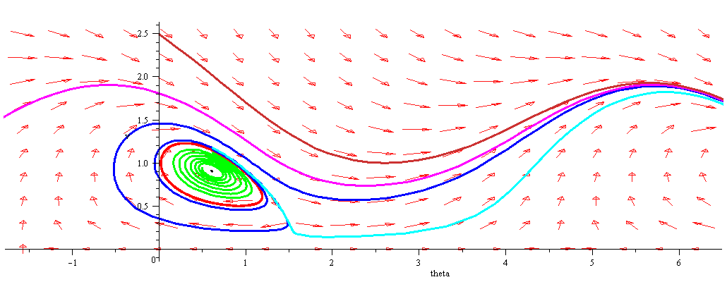
Above we see several things going on. We'll first discuss this in the phase plane, then turn to the actual behaviour of the corresponding glider.
There are three special, periodic solutions:
Then there are three broad classes of solutions.
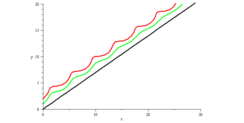
What does this tell us about the actual glider flight? Let's examine the solutions above in the ![]() coordinates. First, let's look at the black (fixed), red (unstable limit cycle) and green solutions.
coordinates. First, let's look at the black (fixed), red (unstable limit cycle) and green solutions.
| > | DEplot(phug, [theta(t), v(t), x(t), y(t)], t=0..40,
[ [theta(0)=0.60877, v(0)=0.904, x(0)=0, y(0)=0], # black [theta(0)=0.60877, v(0)=1.12, x(0)=0, y(0)=1], [theta(0)=0.60877, v(0)=1.151355, x(0)=0, y(0)=2]], # red scene=[x,y], linecolor=[black,green,red], view=[0..30, 0..20], scaling=constrained); |
Here, the black solution corresponds to a glider which starts off with exactly the right initial velocity and angle to climb at a constant rate and angle (about 35 degrees, or .60877 radians).
In the green solution, the plane had the same initial angle, but a velocity a little too high. Because of the greater velocity, it begins to climb, then it loses velocity and the angle decreases, which causes it to pick up speed again, and so on. However, as time progresses, each of these oscillations become less and less, and eventually it limits on the same behaviour as the black solution: climbing with a constant rate. The same would have happened if the velocity had been a little too low, or the angle a little off, etc, because the black solution is a sink, attracting nearby solutions.
The red solution, on the other hand, repeats its oscillation pattern. The velocity is too high, then too low, then too high, and so on, and never stabilizes towards the black fixed soution.
Now let's look at the solutions outside the red limit cycle.
 |
| > | DEplot(phug, [theta(t), v(t), x(t), y(t)], t=0..50,
[[theta(0)=0.60877, v(0)=1.151355, x(0)=0, y(0)=0], # red [theta(0)=0.60877, v(0)=1.16088, x(0)=0, y(0)=0], #blue [theta(0)=0.60877, v(0)=1.1752924, x(0)=0, y(0)=0] #cyan ], scene=[x,y], numpoints=200, linecolor=[red,blue,cyan], view=[0..20, 0..15], scaling=constrained); |
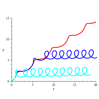
Here all three solutions start out with almost exactly the same initial condition, although the blue and cyan ones have a slightly larger velocity than the red.
The red solution is a climbing solution, but with a nausea-inducing oscillation. The dark blue solution follows the red solution for a few oscillations, but the size of them gets greater and greater until the glider begins a steady looping behaviour. The cyan solution has a slightly higher initial velocity than the blue, and it begins its looping almost immediately. Note that the blue and cyan solutions have almost exactly the same behaviour in the end, just with one happening higher than the other.
 |
Finally, we examine the limiting looping solution (magenta):
| > | DEplot(phug, [theta(t), v(t), x(t), y(t)], t=0..55,
[ [theta(0)=0.60877, v(0)=1.16088, x(0)=0, y(0)=0], [theta(0)=0.60877, v(0)=1.1752924, x(0)=0, y(0)=0], [theta(0)=-2*Pi,v(0)=1.810192, x(0)=0, y(0)=8], # magenta [theta(0)=0, v(0)=4, x(0)=0, y(0)=12] ], scene=[x,y], numpoints=200, linecolor=[blue,cyan,magenta,orange], view=[-1..19, 0..15], scaling=constrained); |
 |
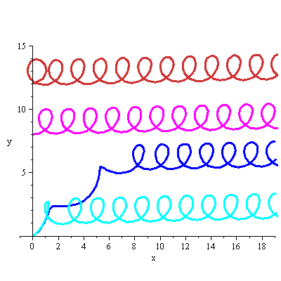
Here we see that despite initially different behaviour, all of the various possibilities limit on the same looping behaviour which corresponds to the magenta solution. If you look closely, you'll see that because of the large initial velocity, the first loop of the orange solution is bigger; however, it quickly becomes the same as all the others.
In summary, we see that nearly every solution eventually becomes a looping solution (like the magenta one) or a climbing solution (like the black one). The red solution (climbing oscillation) is the boundary between these two ultimate fates.
(I ignored the solution which stalls out on the first loop in the x-y plane-- the cyan solution comes close to this, but doesn't quite. Do you see why it is impossible to do one loop then stall on the second one? However, a solution can oscillate any number of times and then stall.).