>	data:=[[1,2], [2,2], [5,6], [7,9], [8,10]];

 

(1)

 

>	err := (f, p) -> abs( f(p[1]) - p[2]);

 

(2)

 

>	dist:= h-> sum( err(h,data[i]), i=1..nops(data));

 

(3)

 

>

 

>	dist(x->x+1);

 

(4)

 

>	dist(x->2*x+1);

 

(5)

 

>	seq(dist(x->x+j),j=-2..8);

 

(6)

 

>	seq([j,dist(x->x+j)],j=-2..8);

 

(7)

 

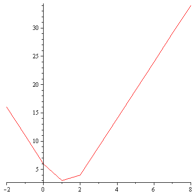
>	plot( [seq([j,dist(x->x+j)],j=-2..8)] );

 

>	mbToDist := (m,b) -> dist(x->m*x+b);

 

(8)

 

>	mbToDist(1,1);

 

(9)

 

>	mbToDist(1.01,1);

 

(10)

 

>	mbToDist(1,1.02);

 

(11)

 

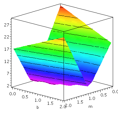
>	plot3d(mbToDist(m,b),m=0..2,b=0..2,axes=boxed,style=patchcontour);

 

>	diff(mbToDist(m,b),m);

 

(12)

 

>	diff(mbToDist(m,b),b);

 

(13)

 

>

 

Oh, ick! abs value isn't differentiable.   

Try something else. 

>	err2 := (f, p) -> ( f(p[1]) - p[2])^2;

 

(14)

 

>	dist2:= h-> sum( err2(h,data[i]), i=1..nops(data));

 

(15)

 

>	mbToDist2 := (m,b) -> dist2(x->m*x+b);

 

(16)

 

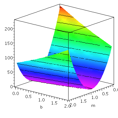
>	plot3d(mbToDist2(m,b),m=0..2,b=0..2,axes=boxed,style=patchcontour);

 

>	diff(mbToDist2(m,b),m);

 

(17)

 

>	diff(mbToDist2(m,b),b);

 

(18)

 

>	solve({diff(mbToDist2(m,b),m)=0,diff(mbToDist2(m,b),b)=0}, {m,b});

 

(19)

 

>	with(plots):

 

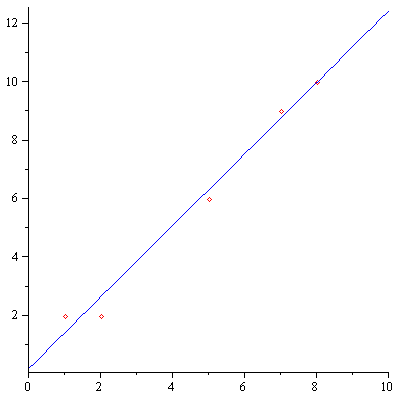
>	display( [ plot(data,style=point, color=red),           plot(38*x/31 + 5/31,x=0..10,color=blue)]);

 

>	CurveFitting[LeastSquares](data,x);

 

(20)

 

>

 

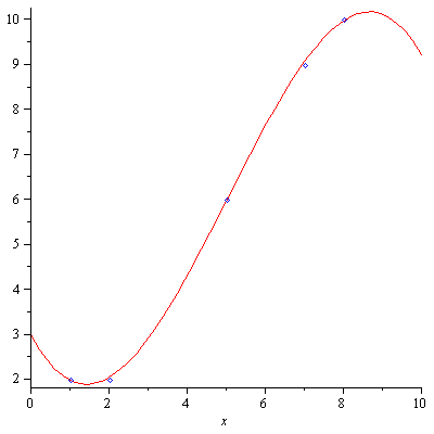
Let's try to find a close cubic instead. 

>	cubdis:=(a,b,c,d) -> dist2(x->a*x^3+b*x^2+c*x+d);

 

(21)

 

>	cubdis(1,2,3,4);

 

(22)

 

>	cubdis(0,0,38/31,5/31);

 

(23)

 

>

 

Find the best values for a,b,c,d that fit a cubic. 

>

 

>	diff(cubdis(a,b,c,d),a);

 

(24)

 

>

 

Just to make it more explicit what we are doing (this isn't necessary), we're going to write out EXACTLY what the function we are minimizing is, so that you can see it is quadratic and so has a unique minimum. 

First, dist2data is the distance from the function h to our 5 points (ie, the sum of the squares of the vertical distance h(x)-y at these 5 points). 

>	dist2data:= unapply(sum( (h(data[i][1])-data[i][2])^2, i=1..nops(data)),h);

 

(25)

 

We want to find a good cubic, so let's give the generic cubic a name 

>	mycubic:=x->a*x^3+b*x^2+c*x+d;

 

(26)

 

Here is the "distance" between the generic cubic and our 5 points.  Note that it depends on a,b,c, and d. 

>	thedist:=dist2data(mycubic);

 

(27)

 

Each of the 4 partials is linear in the 4 variables. 

>	diff(thedist,a);

 

(28)

 

>	ans:=solve( {diff(thedist,a)=0, diff(thedist,b)=0, diff(thedist,c)=0, diff(thedist,d)=0}, {a,b,c,d});

 

(29)

 

So that I don't have to retype, I'm going to use assign. 

>	assign(ans);

 

now a, b, c, and d refer to those specific values. 

>	mycubic(x);

 

(30)

 

>	thedist(mycubic);

 

(31)

 

>	display([plot(mycubic(x),x=0..10),plot(data,style=point,color=blue)]);

 

If I want to use a as a variable again, I need to unassign it: 

>

a,b,c,d;

 

(32)

 

>	unassign('a','b','c','d');

 

>

a,b,c,d;

 

(33)

 

>