>
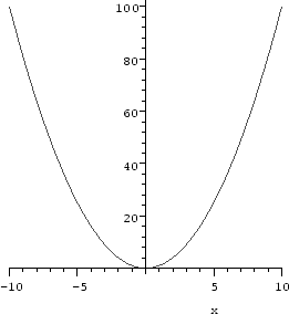
  plot(x^2, x=-10..10);

Maple displays the graph of the function x2 from x = - 10 to x = 10 as requested. In the worksheet interface, clicking the right mouse button on the graph pops up a menu with various options which allow you to manipulate your graph, and/or change its appearance in a suitable way. Clicking the left button ``selects'' the graphic, drawing a black box with ``handles'' around it. You can drag the mouse button on these to resize the plot. Also, the coordinates of the point where you clicked appear in the upper left of the worksheet. Selecting a graphic also changes the context bar: shortcuts for manipulating the axes, aspect ratio, and plotting style appear as buttons along the top.
The basic syntax of the plot command is
>
  plot(f,range);
where f is the expression to be plotted and range is the range
of the parameter(s) for which you would like to see the plot of f. In
the example above, we indicated the range of x by
x=-10..10. Maple automatically chooses a scale on the vertical
axis. There are many options to the plot command; while we will
mention a few of them, the on-line help system has all the details.
Try both of the two similar plot commands below:
>
  plot(x^2-x, x=-1..2, y=-1..2);
  plot(x^2-x, x=-1..2,   -1..2);
In both cases, the plot is displayed for values of y between -1
and 2, but in the first, the variable y is explicitly named
in the command, and the vertical axis gets a label. Whenever you are
plotting an expression, the variable in the domain of the function
must be specified.
>
  slope:=(x1,y1,x2,y2)->(y2-y1)/(x2-x1);
  m:=x->slope(1,1,x,x^2);

We now define the equation of the lines passing through (1, 1) and (x, x2)
for x = 2, 3, 4, 5 and plot the four lines together with the function x^2.
>
  line1:=m(2)*(x-1)+1;
  line2:=m(3)*(x-1)+1;
  line3:=m(4)*(x-1)+1;
  line4:=m(5)*(x-1)+1;
  plot(x^2,line1,line2,line3,line4,x=-3..6);

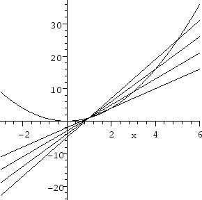
Observe that the expressions to be
plotted are enclosed in braces { }. Besides specifying the
range on which x varies as done above, you can also specify and label
the y range proceeding exactly in the same manner as when plotting a
single function.1.13
plot command is very powerful, and you should look for details about
it using the online help facility; the command ?plot will bring this
up. There are also several related pages, and some instructive example
worksheets that are well worth looking at.
To make you aware of some of its features, we will discuss a few of them here:
>
  points:=[[1,2],[1.5,1],[2,-1],[2.5,0.5],[3,1],[3.5,0.6],[4,0.2]]:
  plot(points,style=POINT);
If style=POINT is replaced by style=LINE, the dots will be
connected by segments of lines. In the worksheet interface, you can switch
from one style to the other by first clicking the left mouse button on the
graph, and then hitting the relevant button on the buttonbar.
On the other hand, if the points result from evaluating an expression at
several values of x, you can use plot in its usual form, but
specifying style=POINT:
>
  plot(x^2,x=-2..2,style=POINT);
Approximately 50 points will be plotted this way. You may notice that
they will not usually be equally spaced, but concentrated in areas where the
graph curves more. You can insist that more
points be plotted by using the numpoints option:
>
  plot(x^2,x=-2..2,style=POINT,numpoints=150);
plots. For basic plotting, there are two
commands from this library that are especially useful. They are
textplot and display. To
load these commands into the computer memory, execute the statement
>
  with(plots,textplot,display);
display command is useful to combine different kinds of plots into
one picture. You can merge standard plots of expressions, plots of points,
plots of text (This is the utility of textplot: to label things),
and animations. In the next example, we combine the point plot of the
variable points defined above with a plot of sin(3*x). We
first define them as different plots and then display them together. Note
that except for the third command, we end with a colon (:) in order to
suppress the Maple output.
>
  plot1:=plot([points],style=POINT):
  plot2:=plot(sin(3*x),x=0..4):
  display(plot1,plot2,view=[0..4,-1..2]);
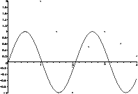
view option controls the horizontal and vertical ranges
to be displayed.
You can attach labels to your plots by combining textplot with
display. The basic syntax of textplot is to use it with an
argument of the form [a,b,'name'] which places the word name inside
the quotes on the plot so that it is centered at the point (a, b).
For example:
>
  y:=(1+x^2)*exp(-x^2/2): d:=diff(y,x):
  F:=plot(y,d,x=-3..3):
  G:=textplot([1,1,'function'],[0.75,0.45,'derivative']):
  display(F,G);
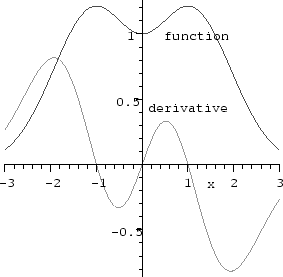
We end with a word about plotting functions (as opposed to expressions), and
a situation in which it is a good idea to do so. Sometimes you will have a
relationship that you want to plot in the form of a function rather than an
expression:
>
  f:=x->x^3*exp(-x):
In this situation, you can plot f(x) as explained above. Alternatively,
you may use:
>
  plot(f, 0..3);
The two ways of plotting a function should not be confused. Neither of the
following two statements will work correctly:
>
  plot(f(x), 0..3);
![]()
>
  plot(f, x=0..3);
As you see, the first gives an error; the second gives a plot with nothing
plotted on it.
If you have a function defined using an if-then clause, you must use
the function plotting command:
>
  f:=x-> if x<3 then x+1 else -x^2+13 fi:
  plot(f(x),x=0..5);
![]()
The error resulted because Maple attempts to understand the expression
f(x) before it has a value for x. One way around
this1.14is to use the command
>
  plot(f, 0..5);
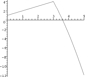
f is probably
continuous but not differentiable at x=3.