Fitting a line to data

Suppose that we are in the situation described above, with m = 1, and that the function f is a polynomial of degree 1. Hence, the number of parameters is two, and for convenience we write

f (x) = mx + b ,

in order to interpret the parameters m and b as the slope and y-intersect of the graph of f. We have data points (x₁, y₁), ..., (x_n, y_n). Our problem is to find the values of m and b will best fit this data. Or to put it simply and geometrically, what is the straight line that best fit the information contained in the data (x₁, y₁), ..., (x_n, y_n)?.

The contribution to the error function coming from the i^th piece of data, (x_i, y_i), is given by (mx_i + b - y_i)², and therefore, the total error is

E(m, b) = $$\sum_{i=1}^{n}$$(mx_i + b - y_i)² .

The problem then becomes that of searching for the values of m and b where the error E(m, b) achieves a minimum. Let us solve this problem using Maple.

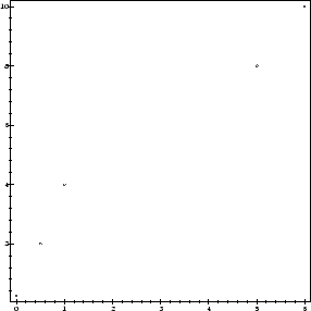
First, let us type in some data to try to fit our line to:

> 
   pts := [ [0,0.25], [1/2,2], [1,4], [5,8], [6,10] ]:

> 
   plot(pts, style=point, axes=boxed);

In order to solve the problem at hand, we could use Maple's built-in regression package to find the answer, but that would not help much in explaining what is going on. However, let us do this anyway.

We can use the LeastSquares command from the CurveFitting package^2.3

> 
  CurveFitting[LeastSquares](pts,x);

This says that the best values of m and b are m = 1.431451613 and b = 1.271370968, respectively. Now let's go through the steps ourselves, to better understand the process.

First, we define the error function according to the data points to fit that we have. Notice again that this function is the square of the distance from the line to the data:

> 
  E := (m,b,pts)-> sum( ((m*pts[i][1]+b)-pts[i][2] )^2, i=1..5);

For example, had we guessed that the line y = 2x + 1 is the answer to our problem, we could compute the distance:

> 
  E(2,1,pts);

However, decreasing m and increasing b produces a smaller value of E, so that guess cannot be the best fit:

> 
  E(1.5,1.2,pts);

We want to minimize the error function. Since minima of differentiable functions occur at critical points, we begin by solving for the values of (m, b) which annihilate the two partial derivatives. Notice that Maple happily computes partial derivatives:

> 
  diff( E(m,b,pts), m);

We may then ask Maple to solve the system of equations obtained by equating the two partial derivatives by

> 
  solve(  diff( E(m,b,pts), m)=0, diff( E(m,b,pts), b)=0 , m,b);

Maple thus finds only one solution, and not surprisingly, it coincides with the solution found using the built-in version.

If we now want to use this values of m and b without retyping it, one way to do that is to use the command assign(%) to let b and m be given these constant values.^2.4

> 
  assign(

Maple executes this assignment silently, without reporting the assignment. However, now both m and b have the assigned values:

> 
  m;

> 
  E(m,b,pts);

The value of E(m, b, pts) calculated above, is the value of E when (m, b) is the critical point found earlier.

We may visualize how good our fit is, using plot to display the data points and the fit line on the same graph. We load the plots package, so that we can use display:

> 
  with(plots):
  display(plot(m*x+b, x=-1..6.5, axes=boxed),
           plot(pts, style=point)):

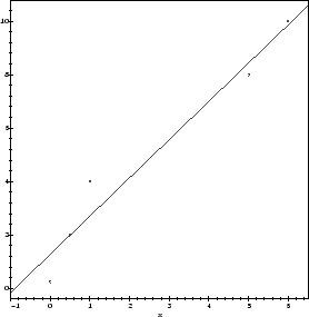
Notice that at this point, m and b have constant values previously assigned to them, the values producing the minimum of E up to 9 decimal places. Let us try to verify that our solution is indeed correct, via an argument which is independent of the one described above.

Geometrically, the error function E is the square of the Euclidean distance between m$\vec{x}$ + $\vec{b}$ and the vector $\vec{y}$, where $\vec{x}$ = (x₁, x₂,..., x_n), $\vec{b}$ = (b, b,..., b) and $\vec{y}$ = (y₁,..., y_n). Clearly then, the best fit is achieved when the coefficients m and b are chosen so that m$\vec{x}$ + $\vec{b}$ is the orthogonal projection of the vector $\vec{y}$ onto the subspace of $\R^{n}$ spanned by $\vec{x}$ and (1, 1,..., 1). That is to say, the best fit occurs when the vectors $\vec{y}$ - (m$\vec{x}$ + $\vec{b}$) and m$\vec{x}$ + $\vec{b}$ are perpendicular to each other. Let us verify this:

> 
  sum( (pts[i][2]-m*pts[i][1]-b)*(m*pts[i][1]+b),i=1..5);

The resulting inner product is not quite zero, but the first non-zero digit of its decimal expansion occurs in the eighth decimal place. This is because the calculations were only done with finite precision, and the discrepancy above is attributable to round-off errors..

As a final remark, we observe that if you now execute the command diff( E(m,b,pts),m ), you will obtain an error. This is due to the fact that m and b are constants at this point, and not independent variables. If you would like to continue making use of the function E(m, b, pts) for general m and b, you will have to unassign the values of m and b first:

> 
  m := 'm':
  b := 'b':

Footnotes

... package^2.3

As we noted before, the CurveFitting package was introduced in Maple 7. Earlier versions of Maple (as well as Maple 7) can accomplish the same thing using the fit command from the stats package, as follows.
with(stats):
fit[leastsquare[[x,y]]]([[ pts[i][1] $i=1..5], [ pts[i][2] $i=1..5]]);
As you can see, the syntax is a little different.