Dealing with the Singularity

The phugoid equations

$$\dot{\theta}$$ = $${\frac{v^2 - \cos\theta}{v}}$$        $$\dot{v}$$ = - sin$$\theta$$ - Rv²

run into trouble when v = 0, because $\dot{\theta}$ becomes infinite as v $\rightarrow$ 0. Since there are very few solutions for which v is ever zero, you might be tempted to ignore this issue, as we have done so far. But in fact, since we are solving the system numerically (rather than exactly), we run into problems even when v is merely small. So far, we have taken care to avoid such situations. But now let's throw caution to the wind, and see what happens.

> 
  R:=0.3:
  DEplot([diff(theta(t),t)=(v(t)^2 - cos(theta(t)))/v(t), 
          diff(v(t),t)    = -sin(theta(t)) - R*v(t)^2], 
    [theta,v], t=0..10, 
    [seq([theta(0)=0,v(0)=2+i/10],i=0..10)],
    theta=-1.5..3, v=-0.05..3, title="R=0.3",linecolor=black,stepsize=0.1);

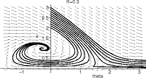
Something looks very wrong with the solution which starts at $\theta$ = 0, v = 2.5. Notice how the solution makes a sharp turn, heading in a completely different direction from the vector field. Why is this happening?

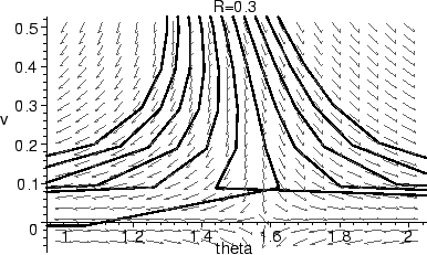
Just to verify that it isn't a fluke, let's examine several solutions with initial conditions $\theta$(0) = 0 and 2.4 < v(0) < 2.6, looking in the problem area. We'll use obsrange=false to tell Maple we want it to continue computing the solutions, even when they go outside of the viewport.

> 
  DEplot( [diff(theta(t),t) =  (v(t)^2 - cos(theta(t)))/v(t),
           diff(v(t),t)     =  -sin(theta(t)) - R*v(t)^2 ], 
    [theta,v], t=0..10, 
    [seq([theta(0)=0,v(0)=2.4+.02*i],i=0..10)],
    theta=1..2, v=-0.05..0.5, obsrange=false,
    title="R=0.3",linecolor=black,stepsize=0.1);

Even worse! Not only does the solution for v(0) = 2.5 go the wrong way, the one with v(0) = 2.52 also turns the wrong way, crossing over another solution. Since our equations are autonomous, this is never supposed to happen.

We can remedy this by decreasing the stepsize significantly. Decreasing the stepsize by a factor of 10 (to 0.01) in the above example gives solutions which do the right thing. But a significant price in computation must be paid, and this doesn't really solve the problem. There are other initial conditions nearby which lead to the same trouble.

In order to decide how to fix the problem, we must first understand what is going wrong. The first problem we noticed happened for a solution with $\theta$(t_i) $\approx$ 1.44, v(t_i) $\approx$ 0.09, using a stepsize h = 0.1. Since Maple is using a Runge-Kutta method as described in §4.2, let's calculate what is happening.

Recall that in Runge-Kutta, we evaluate the vector field at four points, and average them together to get the next point. We denoted these vectors as $\vec{k}_{\ell}^{}$, $\vec{k}_{c}^{}$, $\vec{k}_{m}^{}$, and $\vec{k}_{r}^{}$. Since we have to calculate the vector field at four points, we'll write a little function to do this for us, and use the fact that Maple lets us do aritmetic on lists as though they are actual vectors; that is, we can add them and multiply by scalars.^3.7

> 
  h:=0.1:
  VF:=p->[(p[2]^2 - cos(p[1]))/p[2], -sin(p[1])-R*p[2]^2]:
  

  p:=[1.44, 0.9];
  k[l]:=VF(p);
  k[c]:=VF(p+h/2*k[l]);
  k[m]:=VF(p+h/2*k[c]);
  k[r]:=VF(p+h*k[m]);
  step:=h/6*(k[l] + 2*k[c] + 2*k[m] + k[r]);

The problem here is the vector $\vec{k}_{r}^{}$, which has a huge $\dot{\theta}$ component, and points in a different direction from the others. This happens because k_r is the value of the vector field calculated at $\theta$ $\approx$ 1.35, v $\approx$ - 0.00315. Not only is the value of v very small here (giving a huge $\dot{\theta}$ component), it is outside the range of allowed values, and the vector field points the wrong way. Similar problems will occur for any solution which comes too close to the v = 0 axis with v(t) decreasing.

Now the question is how to avoid this? One not very satisfying answer is just to use a very small step size. But the problem with this idea is that we then must do a huge amount of computation, even when the vector field is behaving nicely.

A better solution is to use an adaptive stepsize: when the vector field is ``nice'', we can use a large step, and when the vector field is being troublesome, we use a small step. Maple has such methods built in to it, such as the Runge-Kutta-Fehlberg method, which we can use by appending method=rkf45 to the list of options to DEplot.

Sometimes, it is not always possible to change the numerical method. In the case of the phugoid, we can accomplish the same goal (in fact, gain something extra) by adjusting the length of the vectors that make up the vector field.

If we think of our solution curves as being parametric curves with tangent vectors which coincide with the vector field, then changing the lengths of the vectors (but not their direction) will not change the solution curves, only the parameterization. That is, we can rescale time so that the vectors no longer blow up as solutions approach the v = 0 line.

Multiplying each vector by v(t) cancels out the problems in $\dot{\theta}$, and gives a system which has the same solution curves as long as v > 0. Thus, we get the new system

$$\dot{\theta}$$ = v² - cos$$\theta$$        $$\dot{v}$$ = - v sin$$\theta$$ - Rv³        $$\dot{x}$$ = v²cos$$\theta$$        $$\dot{y}$$ = v²sin$$\theta$$

This new system of equations is defined and continuous for all values of v and $\theta$.

Furthermore, if we want to keep track of the original time variable t, we can add a new variable T. In the original, non-rescaled equations, the time could be described as T(t) = t, or equivalently, $\dot{T}$ = 1. After rescaling the vector field by the factor of v, this gives $\dot{T}$ = v.

> 
  R:='R';
  vphug:= [ diff(theta(t),t) =  v(t)^2 - cos(theta(t)),
            diff(v(t), t)    = -v(t)*sin(theta(t)) - R*v(t)^3, 
            diff(x(t), t)    =  v(t)^2 *cos(theta(t)),
            diff(y(t), t)    =  v(t)^2 *sin(theta(t)),
            diff(T(t), t)    =  v(t) ]:
  

  R:=0.3:
  

  DEplot(vphug, [theta, v, x, y, T], t=0..20,
         [seq([theta(0)=0,  v(0)=2+i/10, x(0)=0, y(0)=5, T(0)=0],i=0..10),
              [theta(0)=0,  v(0)=2.51, x(0)=0, y(0)=5, T(0)=0],
              [theta(0)=0,  v(0)=2.52, x(0)=0, y(0)=5, T(0)=0],
           seq([theta(0)=0,  v(0)=2.51+i/1000, x(0)=0, y(0)=5, T(0)=0],i=2..5) ],
         theta=-1.5..3, v=-0.05..3, x=0..10, y=0..5,  T=0..20,
         obsrange=false, linecolor=black, scene=[theta,v], stepsize=0.1);

> 
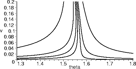
  zoom(

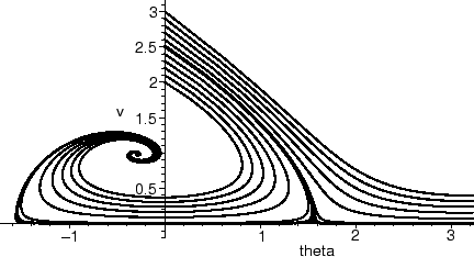
As you can see, using the desingularized equations solves the problems for small values of v.

In addition, we can see additional structure not apparent in the original equations. There are new fixed points at v = 0, $\theta$ = ±$\pi$/2. These fixed points are saddles, as we can see by looking at the Jacobian. In the desingularized equations, the Jacobian is

$$\left(\vphantom{ {\begin{array}{cc} \sin\theta & 2v [2ex] -v\cos\theta & -\sin\theta - 3R v^2 \end{array}} }\right.$$$$\begin{array}{cc} \sin\theta & 2v [2ex] -v\cos\theta & -\sin\theta - 3R v^2 \end{array}$$$$\left.\vphantom{ {\begin{array}{cc} \sin\theta & 2v [2ex] -v\cos\theta & -\sin\theta - 3R v^2 \end{array}} }\right)$$

so the linearization at (${\frac{\pi}{2}}$, 0) is $\left(\vphantom{ \begin{array}{cc} 1 & 0 0 & -1 \end{array} }\right.$$\begin{array}{cc} 1 & 0 0 & -1 \end{array}$$\left.\vphantom{ \begin{array}{cc} 1 & 0 0 & -1 \end{array} }\right)$, and at (- ${\frac{\pi}{2}}$, 0) we have $\left(\vphantom{ \begin{array}{cc} -1 & 0 0 & 1 \end{array} }\right.$$\begin{array}{cc} -1 & 0 0 & 1 \end{array}$$\left.\vphantom{ \begin{array}{cc} -1 & 0 0 & 1 \end{array} }\right)$. These fixed points correspond to the solutions which stall out, and as we surmised earlier, they divide up the qualitative behaviors. The eigenvectors for both of them are parallel to the $\theta$ and v axes, which says that solutions tending to a stall (or leaving one) do so by flying nearly straight up (resp. down) with an angle of $\pi$/2 (resp. - $\pi$/2). Solutions with very small velocity and an angle slightly less than $\pi$/2 flip over rapidly to an angle slightly more than - $\pi$/2 and then begin to increase their velocity.

While it is possible to deduce this behavior from the original equations, it is much more obvious one the singularity is filled in. Similar techniques are used in other branches of mathematics (blowing up a singularity in algebraic geometry, construction of a collision manifold in celestial mechanics) with great success.

Footnotes

... scalars.^3.7

This ability is not present in releases prior to Maple 6, making this computation a little more cumbersome.