Robust fitting

Let us return momentarily to the problem discussed in §3: given some data (x₁, y₁),...,(x_n, y_n), we found the best line that fits it. This was accomplished by measuring the square of the vertical distance from each data point and the line y = mx + b, which led us to consider the error function

E(m, b) = $$\sum_{i=1}^{n}$$(mx_i + b - y_i)² .

The problem was solved by finding the values of m and b where E achieves its minimum.

However, the square of the vertical distance is only one of many reasonable ways of measuring the distance from the data points to the line mx + b. For example, it is perfectly reasonable to consider instead the expression 1 + (mx_i + b - y_i)². If (x_i, y_i) is on the line, this value would be equal to 1, and its logarithm would then be zero. Thus, the function

E(m, b) = $$\sum_{i=1}^{n}$$ln$$\left(\vphantom{ 1 + (mx_i+b-y_i)^2 }\right.$$1 + (mx_i + b - y_i)²$$\left.\vphantom{ 1 + (mx_i+b-y_i)^2 }\right)$$ ,

is also a reasonable way of measuring the distance from the data points to the line y = mx + b, and its minimum would produce a best fit line in this other sense. Similarly, We may argue that the function

E(m, b) = $$\sum_{i=1}^{n}$$$$\left\vert\vphantom{ mx_i+b-y_i }\right.$$mx_i + b - y_i$$\left.\vphantom{ mx_i+b-y_i }\right\vert$$ .

is another reasonable alternative, though this time E is not even differentiable in the region of interest (if a data point (x_i, y_i) happens to be exactly on the line, mx_i + b - y_i = 0 and the absolute value is not differentiable at 0).

There is a priori no particular reason to prefer one error function over another. And for each choice of such we could end up with a problem whose solution exists and produces a line that best fit the data. Then we could compute the value of the error function for the best fit line, value that depends upon the choice of function made. A canonical way of choosing the best error function could be that for which this number is the smallest. But finding such a function is quite a difficult, if not impossible, problem to solve. If we limit our attention to linear estimators, in a sense to be explained in the last section of this chapter, the solution obtained in §3 is optimal. In here, we pursue further the problem of finding the best fit according to the two error functions introduced above.

Notice that if $\epsilon_{i}^{}$ = mx_i + b - y_i, data with large errors $\epsilon_{i}^{}$ excert a huge influence on the original error function of §3 (because we use $\sum$$\epsilon_{i}^{2}$). The two error functions mentioned above grow linearly (or sub-linearly) with |$\epsilon_{i}^{}$|, causing the tails to count much less heavily. We will see this when comparing the different results.

In order to solve the problem now at hand, we first generate some ``noisy'' data. We load the routines in lsq_data.txt:

> 
  read(`lsq_data.txt`);

The data and its graphical visualization can then be obtained by:

> 
  pts:=bad_line_pts():

> 
  plot(pts,style=point,symbol=box);

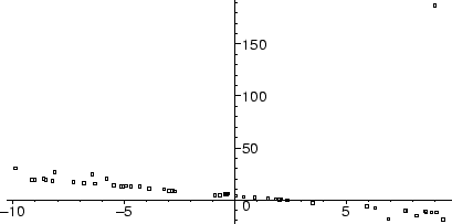
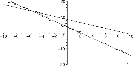
You should notice that while most of the data lies fairly near a line, there is one point which is extremely far away from the rest of the data.

In order to compare results, let us first find the line given by least squares. First, we define a function $\epsilon$, which gives the signed vertical distance between a point pt and a line of slope m and intercept b

> 
  epsilon:= (pt,m,b) -> (m*pt[1]+b-pt[2]);

Now we compute the regular least squares fit.

> 
  H:=(m,b,pts)->sum(epsilon(pts[i],m,b))^2,i=1..nops(pts)):
  sol:=solve(diff(H(m,b,pts),m)=0, diff(H(m,b,pts),b)=0,m,b);

> 
  display(plot(pts,style=point,symbol=box),plot(subs(sol,m*x+b),x=-10..10),
          view=-20..20);

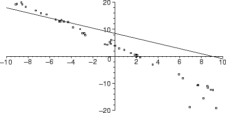
In the above, we restricted our attention to the region -20 < y < 20, where the line and the majority of the data lies. As you can see, the fit to the majority of the data is very poor, because of the influence exerted by the anomalous data point.

Now, let's try again, this time minimizing ln(1 + $\epsilon_{i}^{2}$/2), which behaves like $\epsilon^{2}_{}$ for small errors, but grows very slowly for large ones.

> 
  R:=(m,b,pts)->sum(ln(1+epsilon(pts[i],m,b)^2/2),i=1..nops(pts));

Here's what the functional we want to minimize looks like:

> 
  plot3d(R(m,b,pts),m=-5..0,b=-20..0,style=patchcontour, axes=boxed);

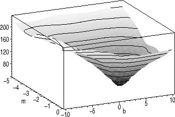
The equations we want to solve are not linear. In fact, they're messy enough that Maple needs some help to find the minimum. By examining the plot and zooming in on the minimum, we can choose an appropriate region.

> 
  plot3d(R(m,b,pts),m=-2..-1.5,b=3..5,view=38..50, axes=boxed);

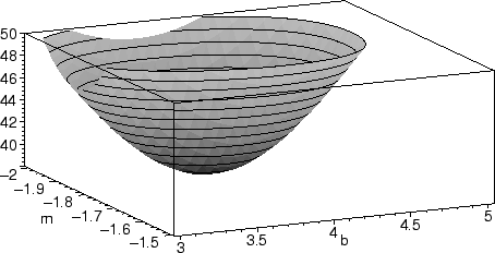
Once we have an appropriate region, we can ask Maple to look for the solution numerically using fsolve.

> 
  rs:=fsolve( diff(R(m,b,pts),m)=0, diff(R(m,b,pts),b)=0,
              m,b,m=-2..-1.5, b=3..5);

And here we can compare the two lines found.

> 
  p := plot(pts,style=point):
  l := plot(subs(sol,m*x+b),x=-10..10):
  s := plot(subs(rs,m*x+b),x=-10..10,color=blue):
  plots[display](p,l,s,view=-20..20);

Let us now try to minimize $\sum$|$\epsilon_{i}^{}$|. Since this function is not even differentiable near $\epsilon_{i}^{}$ = 0, we have to work harder to get less.

> 
  A:=(m,b,pts)->sum(abs(epsilon(pts[i],m,b)),i=1..nops(pts));

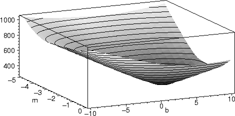
Displaying the graph of this function gives us an idea about where its minimum lies:

> 
  plot3d(A(m,b,pts),m=-5..0,b=-10..10,style=patchcontour, axes=boxed);

But coercing Maple into finding a numerical approximation to it is not so easy. There are reliable and efficient ways to determine the location of the minimum to any precision (at least given some hints), but they are inappropriate for the scope of this chapter, and will not be considered here. Instead we may zero in on the minimum by looking at where the lowest point is and repeatedly restricting the domain. After several iterations, we get the following.

> 
  plot3d(A(m,b,pts),m=-1.0875..-1.0872,b=3.817..3.8178, axes=boxed);

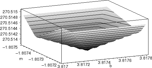
This leads us to a choice of m = - 1.80733, b = 3.8174 as our ``best'' line. This is almost (but not quite) the same line found using our distance R(m, b).