Fitting a circle

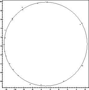
In a slightly different vein, suppose that the data points {(x_i, y_i)} lie near a circle of unknown center and radius. Note that if we did know the center, this problem would be very simple: the desired radius would be the average distance from the points to the center. If you don't think very hard, you might suspect that the desired center would be very near the center of mass of the points {(x_i, y_i)}, but this will only be the case if the points are evenly distributed around the circle.

Instead, we can come up with a function that measures the error between an arbitrary circle and our data points.

Recall that the general equation of a circle centered at (a, b) with a radius of r is

(x - a)² + (y - b)² = r².

Unlike the previous cases, there is no independent variable. (Note that we could try to fit y_i $\simeq$ b±$\sqrt{r^2 -(x_i-a)^2}$, but not only would the resulting equations be messy, this would bias things very badly; do you see why?). Nevertheless, we press on.

One reasonable measure of the distance between the points and a circle is the ``area difference'', that is

E(a, b, r) = $$\sum_{i}^{}$$$$\left(\vphantom{ (x_i-a)^2 + (y_i-b)^2 - r^2 }\right.$$(x_i - a)² + (y_i - b)² - r²$$\left.\vphantom{ (x_i-a)^2 + (y_i-b)^2 - r^2 }\right)^{2}_{}$$.

One difficulty with this is that E is not quadratic in a, b, and r. However, Maple is able to solve the resulting equations anyway.

We assume here that there is a routine called circle_pts which gives us points which lie near a circle of unknown radius and center. The one we use here is similar to that in §4, and is defined in lsq_data.txt.

> 
  cpts:=circle_pts():
  epsilon:=(pt,a,b,r) -> (pt[1]-a)^2 + (pt[2]-b)^2 -r^2;

> 
  E:= (a,b,r,pts) ->   sum( epsilon(pts[i],a,b,r)^2,  i=1..nops(pts));

> 
  sol:= solve(diff(E(a,b,r,cpts),a)=0,
                diff(E(a,b,r,cpts),b)=0,
                diff(E(a,b,r,cpts),r)=0,
              a,b,r);

Here we find a number of critical points for the function E, but from physical considerations, the only reasonable choice is the circle for which r > 0.

This is the seventh entry in the above list, so we could refer to it just by sol[7]. However, with a different set of data, it might be the second solution, or the fourth, etc. To ensure that we always get the right one, no matter what the order is, we can use Maple's select command to pull out the one with r > 0. This looks more daunting than it really is: we just define a function that returns true if that r > 0 for that solution, and false if not. Then select returns only those elements for which the function is true. We need to use op, because we have a list of sets, and we just want the one answer.

> 
  goodsol:=op(select(s->if (subs(s,r)>0) then true else false fi,sol));

In order to see the fit, we plot the points and the circle. Note that we represent the circle parametrically, and use subs to substitute the desired solution.

> 
  display(
    plot(cpts,style=point,scaling=constrained,axes=boxed),
    plot(subs(goodsol,[a+r*cos(t),b+r*sin(t),t=0..2*Pi]))
  );

The fact that there is only one interesting critical point is no accident, however. If we let k = a² + b² - r², then the resulting error function H(a, b, k) = E(a, b,$\sqrt{a^2+b^2 -k}$) is quadratic in a, b, and k, and so we really only need to solve a linear system. It is easy to check that this new functional H still satifies all the criteria we wanted (that is H(a, b, k) = 0 if and only if all the data points lie on the circle C(a, b, k), H is non-negative, and it is smooth), so fitting a circle becomes a linear problem after all. The reader should verify that, in fact, the unique minimum of H corresponds exactly to the critical points the original function E for which r$\ne$ 0.

The interested reader might want to consider a similar approach to fitting other conic sections, such as an ellipse or a hyperbola, to given data. Do you expect to be able to make the problem linear, as in the case of the circle?