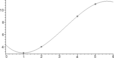
> data:=[[1,3],[2,4],[4,9],[5,11]]:with(CurveFitting): cubfit:=PolynomialInterpolation(data,x);
First, we will look at the situation where we the data points are assumed to be known exactly (or at least to good enough precision that we ignore any errors), and we want to find a curve of some type is chosen that passes through each of the data points. This practice is called interpolation. In the latter part of this chapter (beginning with §2), we will relax the restriction that the curve pass exactly through the points.
Of course, there are serious restrictions involved in interpolation. Since a line is determined by two points, if we have more points, we must either use a higher degree polynomial, or use several line segments. If we have n data points we wish to interpolate, either we can fit a polynomial of degree n - 1 or find n - 1 line segments which ``connect the dots''. We'll address both of these in this section, as well as a method which is a cross between the two approaches.
Given n data points (x1, y1),(x2, y2),...,(xn, yn), there is a unique polynomial of degree n - 1 passing through them. Finding this polynomial is just a matter of solving the n linear equations for the coefficients. For example, suppose we have 4 data points (x1, y1), (x2, y2), (x3, y3), and (x4, y4). There is exactly one degree 3 polynomial p(x) = ax3 + bx2 + cx + d which passes through all four points. Plugging in our data yields the equations
| ax13 + bx12 + cx1 + d | = | y1 |
| ax23 + bx22 + cx2 + d | = | y2 |
| ax33 + bx32 + cx3 + d | = | y3 |
| ax43 + bx42 + cx4 + d | = | y4 |
Maple 72.1 has a built-in command called PolynomialInterpolation to do this automatically for us, as part of the CurveFitting package. We'll do a brief example.
with(CurveFitting):
cubfit:=PolynomialInterpolation(data,x);
>
data:=[[1,3],[2,4],[4,9],[5,11]]:
![]()
>
  plots[display](
    plot(data,style=point,color=black,symbol=BOX),
    plot(cubfit,x=0..6,thickness=2));

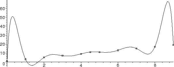
That seems to have worked pretty well. However, we should remark that polynomials are somewhat inflexible: minor variations in the data can have drastic effects on the behavior between the points. To emphasize this, we'll generate 10 points along the line y = 2x + 1, with one more point in the middle that is a bit above the line.
>
  data2:=[seq([i,2*i+1],i=0..4),[9/2,11],seq([i,2*i+1],i=5..9)];
![]()
>
  plots[display](
    plot(data2,style=point,color=black,symbol=BOX),
    plot(PolynomialInterpolation(data2,x),x=0..9,thickness=2));

This doesn't look much like a straight line, does it? Even though there is only one data point which is 1 unit above the line y = 2x + 1, at x = 1/2 the polynomial is about 50 units above this line.
As we said at the start of this section, another choice is not to use a single function, but to use several segments which connect the dots. The result would be a piecewise-affine function consisting of several line segments defined on a number of intervals. In the example using data2 from the previous section, this function would be

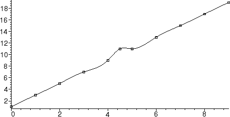
Although writing a maple procedure to figure this out for us would not be hard, such a piecewise affine curve is a version of something called a spline, which we will discuss more soon. This type of connect-the-dots curve is a linear (or degree 1) spline, and Maple can find it using the Spline command out of the CurveFitting2.2 package.
>
  lspline:=Spline(data2,x,degree=1):
>
  plots[display](
    plot(data2,style=point,color=black,symbol=BOX),
    plot(lspline,x=0..9,thickness=2));

If we leave off the degree=1, Maple gives us a cubic spline instead:
>
  plots[display](
    plot(data2,style=point,color=black,symbol=BOX),
    plot(Spline(data2,x),x=0..9,thickness=2));

Notice how the cubic spline fits the points about as well as the ``connect-the-dots'' piecewise affine curve, but has no corners. What is this curve that Maple is showing us?
To make a spline, instead of connecting each pair of points by a straight segment, we put in a polynomial of degree d. We must ensure that the polynomial passes through the two endpoints of each segment, but this still leaves us an additional d - 1 conditions per polynomial segment. The entire curve can be made smoother by choosing each polynomial segment so that the first d - 1 derivatives at one endpoint agree with the derivatives of the previous segment. Since there is no segment before the first or after the last, this leaves d - 1 more conditions still to specify. For a ``natural spline'', the high order derivatives at the endpoints are set to zero:
You might think that using higher degree polynomials in between would give a better appearance, but the same issues that arose in earlier begin to show up. Note that if we have n data points, fitting a spline of degree n - 1 is exactly the same as the interpolating polynomial of degree n - 1. Cubic splines are the most widely used, because they look quite smooth to the eye, but have enough freedom that they don't have to wiggle too much in order to pass through each data point. Many computer drawing programs have the ability to fit cubic splines through a set of points.