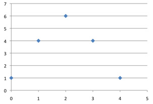
C(4, k)
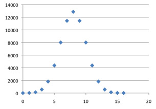
C(16, k)
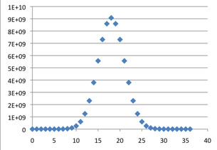
C(36, k)
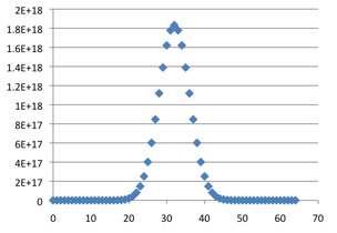
C(64, k)
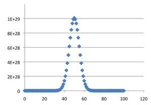
C(100, k)
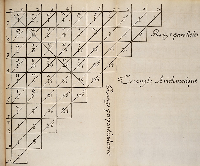
Pascal's triangle from his Traité. In his format the entries in the first column are ones, and each other entry is the sum of the one directly above it, and the one directly on its left. In our notation, the binomial coefficients C(6, k) appear along the diagonal Vζ. Image from Wikipedia Commons.
C(4, k)
C(16, k)
C(36, k)
C(64, k)
C(100, k)
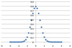
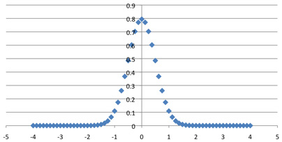
As k varies, the maximum value of C(n, k) occurs at n / 2. For the graphs of C(n, k) to be compared as n goes to infinity their centers must be lined up; otherwise they would drift off to infinity. Our first step in uniformizing the rows is to shift the graph of C(n, k) leftward by n / 2; the centers will now all be at 0.
The estimate mentioned above for the central elements (it comes from Stirling's formula) suggests that for uniformity the vertical dimension in the plot of C(n, k) should be scaled down by 2n / n1/2. Now 2n = (1+1)n = C(n, 0) + C(n, 1) + ... + C(n, n), which approximates the area under the graph; to keep the areas constant (and equal to 1) in the limit we stretch the graphs horizontally by a factor of n1/2.With these translations and rescalings, the convergence of the central portions of the graphs becomes graphically evident:
C(4, k)*2 / 2^4, plotted against (k-2) / 2
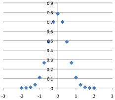
C(16, k)*4 / 2^16, plotted against (k-8) / 4.
C(36, k)*6 / 2^36, plotted against (k-18) / 6.
C(64, k)*8 / 2^64, plotted against (k-32) / 8.
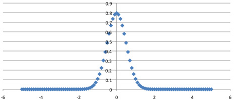
C(100, k)*10 / 2^100, plotted against (k-50) / 10.
Our experiment is an example of the Central Limit Theorem,
a fundamental principle of probability theory (which brings us
back to Pascal). The theorem is stated in terms of random
variables. In this case, the basic random variable X
has values 0 or 1, each with probability 1/2 (this could be the
outcome of flipping a coin). So half the time,
at random, X = 0, and the rest of the time X = 1.
The mean or expected value of X is E(X)
= μ = 1/2 (0) + 1/2 (1) = 1/2 . Its
variance is defined by σ2
= E(X2)-[E(X)]2
= 1/4, so its standard deviation is σ = 1/2. The n-th
row in Pascal's triangle corresponds to the sum
X1 + ... + Xn,
of n random variables, each identical to X.
The possible values of the sum are 0, 1, ..., n
and the value k is attained with probability
C(n, k)/2n.
[So, for example, if we toss a coin four times, and count
1 for each head, 0 for each tail, then the probabilities
of the sums 0, 1, 2, 3, 4 are 1/16, 1/4, 3/8, 1/4, 1/16
respectively.] This set of values and probabilities is called
the binomial distribution with p= (1-p) = 1/2.
Its has mean μn = n/2 and
standard deviation σn = n1/2/2.
In our normalizations we have shifted the means to 0 and stretched
or compressed the axis to achieve uniform standard deviation 1/2.
The Central Limit Theorem is more general, but it states
in this case that the limit of these normalized probability
distributions, as n goes to infinity, will be the normal
distribution with mean zero and standard deviation 1/2. This
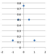
distribution is represented by the function
The normal distribution with μ = 0 and σ = 1/2.
Suppose you want to know the probability of between 4995 and 5005 heads in 10,000 coin tosses. The calculation with binomial coefficients would be tedious; but it amounts to calculating the area under the graph of C(10000, k) between k = 4995 and k = 5005, relative to the total area. This is equivalent to computing the relative area under the normalized curve between (4995-5000) / 100 = -.05 and (5005-5000) / 100 = .05; to a very good approximation this is the integral of the normal distribution function f(x) between -.05 and .05, i.e. 0.0797.
Corrected, May 6 , 2017.
Corrected, Dec 18, 1028.