The mathematics behind quantum computing
The second of two feature columns on this subject.
The Fast Fourier Transform is fast, but not fast enough for
realistic factorization of large numbers. Factoring
an n-bit number would require 3n·2n
operations; that number increases exponentially with n.
This month's column will examine how for a quantum computer
this growth could be made polynomial, and the factorization
problem could become tractable.
Quantum computers
Data in a quantum computer are stored in qubits, and
manipulated by gates.
- A qubit (the name is a contraction of "quantum bit")
is a device whose state can be
represented by a unit vector in a 2-dimensional complex vector space.
In terms of an orthonormal basis, usually designated |0>, |1>,
the state is a0|0> +
a1|1>; here a0 and
a1 are complex numbers satisfying
|a0|2 + |a1|2 = 1.
When the qubit is measured, it reports "0"
with probability |a0|2 and
"1" with probability |a1|2; meanwhile,
the numbers a0 and
a1 are lost.
- Gates have kept their name from an early
mechanistic conception of the flow of information through a
computer. In quantum computation, gates are physical processes
which can be
applied to qubits.
- One-qubit gates. For the operation to be realizable
by a quantum-mechanical
process, the output vector (b0, b1)
must also be a unit vector, and it must
vary linearly with the input vector. In other words,
if V is the vector space of states of the qubit
in question,
the gate
must correspond to a unitary operator on V.
Example: the NOT-gate. This is the simplest example of
a gate that does something.
| NOT-gate: |
| INPUT | OUTPUT |
| |0> |
|1> |
| |1> |
|0> |
|
Here the operator is described by its values on the basis vectors.
Note that NOT takes
 |0>
+
|1>
to itself, so not every vector gets "negated." Also note that this
operation is its own inverse, so it is automatically unitary.
|0>
+
|1>
to itself, so not every vector gets "negated." Also note that this
operation is its own inverse, so it is automatically unitary.
Example: the R-gate. In terms of the basis vectors:
| R-gate: |
| INPUT | OUTPUT |
| |0> |
|0> +
|1> |
| |1> |
|0> – |1> |
|
This gate has been called the "quantum coin-flip." If a qubit starts in state
|0>, after the gate if it is measured it will return 0 with
probability 1/2, and 1 with probability 1/2. This operation is also its
own inverse.
- Two-qubit gates. Now, for physical realizability,
each output state must vary linearly with
each of the
input states. This means that the state space of a pair of
qubits is the
tensor product of their individual
state spaces, and that the gate is represented by
an invertible linear
operator on that tensor product.
Suppose the gate is acting
on the two qubits
qubit with state space basis
|0>,
|1> and
qubit with state space basis
|0>,
|1>. The tensor product
a
 b of a =
a0|0> +
a1|1>
with b =
b0|0> +
b1|1>
is a 4-component object best represented by the matrix:
b of a =
a0|0> +
a1|1>
with b =
b0|0> +
b1|1>
is a 4-component object best represented by the matrix:
In terms of the bases
|0>,
|1> and
|0>,
|1>, the tensor products
| |0> |0> = |
( |
1 0
0 0 |
),
|
|
| |0> |1> = | ( |
0 1
0 0 |
),
|
|
| |1> |0> = | ( |
0 0
1 0 |
),
|
|
| |1> |1> = | ( |
0 0
0 1 |
)
|
|
form a basis for the tensor product of the state spaces.
Example: Controlled-NOT
Such a device inputs 2 qubits, say qubit
and qubit; it
leaves qubit
unchanged and reverses the state of
qubit
whenever qubit is in state
|1>.
| C-NOT gate: |
| INPUT | OUTPUT |
| |0>|0> |
| |0>|1> |
| |1>|0> |
| |1>|1> |
|
| |0>|0> |
| |0>|1> |
| |1>|1> |
| |1>|0> |
|
|
This operation can also be described by saying that the sum
modulo 2 of qubit
and qubit is
stored in qubit,
and that qubit is
carried along to make the operation reversible.
Entanglement
A typical element of the tensor product of the
qubit state space
(basis |0>,
|1>)
and the qubit state space
(basis |0>,
|1>)
will have the form:
c0,0|0>
|0> +
c0,1|0>
|1> +
c1,0|1>
|0> +
c1,1|1>
|1>,
or, written in matrix notation,
subject to the condition |c0,0|2 +
|c1,0|2 +
|c0,1|2 +
|c1,1|2
= 1.
Such an element will in general not be the tensor product
ab
of a =
a0|0> +
a1|1>
and b =
b0|0> +
b1|1>.
In fact, we can write a matrix as
a tensor product
only when the determinant
c0,0 c1,1
– c1,0 c0,1 is 0.
A state in the 2-qubit state space which is not of the form
ab is called an entangled state. Here is why:
- Example of entanglement.
Suppose a 2-qubit register is in the state
|0>
|0> +
|1>
|1>.
When measured, this register has probability 1/2 of being in the
state |0>
|0>, and
probability 1/2 of being in the state |1>
|1>.
If qubit is measured, and found to be in the state
|0>, then when qubit is measured it must also
be in the state |0>. It was entangled.
Note that in the non-entangled case, measurement of
qubit gives no information
about the state of qubit.
Parallel processing in a quantum computer
-
Example 1. Addition modulo 2. This example is elementary
but illustrative. We work with a 3-qubit register
qubit
qubit
qubit
and we modify the Controlled-NOT gate so that
if qubit starts in
state |0>, then its output
state is
the modulo 2 sum of the input
states of qubit
and qubit; the other qubits
remain unchanged. The outputs
when qubit starts in state
|1> will not concern us, except
inasmuch as they make the whole operation unitary. Let us call
this 3-input, 3-output gate a D-gate. In terms of the standard
basis for the tensor product of the three state spaces, it is
described by the table
| D gate: |
| INPUT | | OUTPUT |
|
|0>
|0>
|0>
|
|
|0>
|0>
|0>
|
|
|0>
|0>
|1>
|
|
|0>
|0>
|1>
|
|
|0>
|1>
|0>
|
|
|0>
|1>
|1>
|
|
|0>
|1>
|1>
|
|
|0>
|1>
|0>
|
|
|1>
|0>
|0>
|
|
|1>
|0>
|1>
|
|
|1>
|0>
|1>
|
|
|1>
|0>
|0>
|
|
|1>
|1>
|0>
|
|
|1>
|1>
|0>
|
|
|1>
|1>
|1>
|
|
|1>
|1>
|1>.
|
|
To perform mod 2 addition in parallel, we start with the register in state
|0>
|0>
|0>,
and we apply the R-gate to qubit
and to qubit. This
leaves qubit in state
(|0> +
|1>) and
qubit in state
(|0> +
|1>),
and the register in state
(1/2) |0>
|0>
|0>
+
(1/2) |0>
|1>
|0>
+
(1/2) |1>
|0>
|0>
+
(1/2) |1>
|1>
|0>.
|
We now apply the D-gate once to this register.
The output is
(1/2) |0>
|0>
|0>
+
(1/2) |0>
|1>
|1>
+
(1/2) |1>
|0>
|1>
+
(1/2) |1>
|1>
|0>.
|
Now each qubit,
qubit state pair is entangled
with its mod-2 sum.
If we measure the first two qubits, and
then measure the third, it
will report the sum of the first two measurements.
All of the sums have been carried
out at once! But this is not completely useful, since if we wanted
the program to calculate the sum of a specific
pair, we would need to continue loading and running
until that pair came up in the input. Part of the
subtlety of quantum programming is to structure
algorithms so that the desired information can be extracted
with high probability in a small number of runs.
- Example 2. Another way of reading the output from
our experiment with the D-gate is to measure the output
qubit. This
measurement will yield 0 or 1 with probability 1/2.
Suppose it reads 0. Then if the first two qubits are
measured, they will report 0,0 or 1,1 with equal
probability. The first measurement has collapsed
the state space of the register to allow only these
two possibilities. In other words, it now only contains those
pairs of states whose mod-2 sum is zero.
- More generally, working with an n-qubit
register, n applications of the R-gate (which can be
carried out simultaneously) will produce an equiprobable
superposition of the binary forms of all the numbers from
0 to 2n-1. Any operation that can be encoded
in binary arithmetic can be carried out on all the numbers
simultaneously. Typically the number of steps in this
operation is a low-degree polynomial function of n,
the number of binary places.
This contrast between an exponential range and a polynomial
number of steps is the key to the efficiency of quantum
computation.
The Quantum Fourier Transform
A quantum Fourier transform was first worked out by Peter Shor,
in 1994. This refinement (which corresponds exactly to the
the Radix-2 Cooley-Tukey algorithm)
was discovered, almost immediately afterwards and
independently,
by Richard Cleve, Don Coppersmith and David Deutsch.
Working with a register of
q qubits
qubit0, qubit1, ...,
qubitq–1,
it uses
a combination of the gates Rj (the R-gate applied
to qubitj)
with a set of reversible gates called
Sj,k in Shor's notation.
The gate Sj,k operates on the pair
qubitj, qubitk, with j < k,
as follows:
| Sj,k gate: |
| INPUT | OUTPUT |
| qubitj | qubitk |
| |0> | |0> |
| |0> | |1> |
| |1> | |0> |
| |1> | |1> |
|
| qubitj | qubitk |
| |0> | |0> |
| |0> | |1> |
| |1> | |0> |
| ωk–j|1> | ωk–j|1> |
|
|
where ωk–j = e i π /2k–j. This number is a primitive
(2k–j)-th root of –1.
- Example: the QFT on 3 bits.
For 3 bits, the QFT algorithm specifies the sequence
R2 S1,2 R1 S0,2 S0,1 R0
applied in left-to-right order. Here we abbreviate
|0>|0>|0> as 000, etc.
|
input
000
001
010
011
100
101
110
111
|
after R2
2–1/2 (000 + 001)
2–1/2 (000 – 001)
2–1/2 (010 + 011)
2–1/2 (010 – 011)
2–1/2 (100 + 101)
2–1/2 (100 – 101)
2–1/2 (110 + 111)
2–1/2 (110 – 111)
|
after S1,2 (ω2–1=i)
2–1/2 (000 + 001)
2–1/2 (000 – 001)
2–1/2 (010 +i 011)
2–1/2 (010 –i 011)
2–1/2 (100 + 101)
2–1/2 (100 – 101)
2–1/2 (110 + i111)
2–1/2 (110 – i111)
|
after R1
2–1 (000 + 010 + 001 + 011)
2–1 (000 + 010 – 001 – 011)
2–1 (000 – 010 + i001 – i011)
2–1 (000 – 010 – i001 + 011 )
2–1 (100 + 110 + 101 + 111)
2–1 (100 + 110 – 101 – 111)
2–1 (100 – 110 + i101 – i111)
2–1 (100 – 110 – i101 + i111)
|
|
after S0,2 (ω2–0=e iπ/4 )
2–1 (000 + 010 + 001 + 011)
2–1 (000 + 010 – 001 – 011)
2–1 (000 – 010 + i001 – i011)
2–1 (000 – 010 – i001 + i011 )
2–1 (100 + 110 + e iπ/4 101 + e iπ/4 111)
2–1 (100 + 110 – e iπ/4 101 – e iπ/4 111)
2–1 (100 – 110 + ie iπ/4 101 – ie iπ/4 111)
2–1 (100 – 110 – ie iπ/4 101 + ie iπ/4 111)
|
after S0,1 (ω1–0=i)
2–1 (000 + 010 + 001 + 011)
2–1 (000 + 010 – 001 – 011)
2–1 (000 – 010 + i001 – i011)
2–1 (000 – 010 – i001 + i011 )
2–1 (100 + i110 + e iπ/4 101 + ie iπ/4 111)
2–1 (100 + i110 – e iπ/4 101 – ie iπ/4 111)
2–1 (100 – i110 + ie iπ/4 101 + e iπ/4 111)
2–1 (100 – i110 – ie iπ/4 101 – e iπ/4 111)
|
|
after R0
2–3/2 (000 + 100 + 010 + 110 + 001 + 101 + 011 + 111)
2–3/2 (000 + 100 + 010 + 110 – 001 – 101 – 011 – 111)
2–3/2 (000 + 100 – 010 – 110 + i001 + i101 – i011 –i111)
2–3/2 (000 + 100 – 010 – 110 – i001 – i101 + i011 + i111)
2–3/2 (000 – 100 + i010 – i110 + e iπ/4 001 – e iπ/4 101 + ie iπ/4 011 – ie iπ/4 111)
2–3/2 (000 – 100 + i010 – i110 – e iπ/4 001 + e iπ/4 101 – ie iπ/4 011 + ie iπ/4 111)
2–3/2 (000 – 100 – i010 + i110 + ie iπ/4 001 – ie iπ/4 101 + e iπ/4 011 – e iπ/4 111)
2–3/2 (000 – 100 – i010 + i110 – ie iπ/4 001 + ie iπ/4 101 – e iπ/4 011 + e iπ/4 111)
|
- For 4 bits the QFT algorithm would read
R3 S2,3 R2 S1,3 S1,2
R1 S0,3 S0,2 S0,1 R0;
in general for n bits the Quantum Fourier Transform requires
(n2 + n)/2 operations.
- Note that the Quantum Fourier Transform is not transforming
anything. It gives a way to duplicate through quantum operations
the steps of the Fast Fourier Transform, but without an input
sequence. If the QFT is applied to the equiprobable superposition
of the binary forms of the numbers from 0 to 2n-1, then
in (n2 + n)/2 steps it will produce a
superposition of all the 2n rows of the matrix with
a,c entry ea c i π/2n-1.
More specifically, suppose in our 3-qubit example that
we carry along the input register as
the first 3 qubits
in the computation (this will turn out not be necessary). Then at the
end if the first qubits are measured and
report binary 5, i.e. |1>|0>|1>, the last three
qubits must contain the superposition:
2–3/2 (|0>|0>|0> –
|1>|0>|0> + i|0>|1>|0> – i|1>|1>|0> – e iπ/4
|0>|0>|1>
+ e iπ/4 |1>|0>|1>
– ie iπ/4
|0>|1>|1>
+ ie iπ/4
|1>|1>|1>).
In the "row" corresponding to binary 5,
the coefficient of the state "binary c" is exactly
(2–3/2 times)
e i 5 cπ/4; so that
|0>|0>|0> has coefficient
e i5·0π/4 = 1,
|0>|0>|1> has coefficient
e i5·1π/4 = –e iπ/4,
|0>|1>|0> has coefficient
e i5·2π/4 = i,
etc. By a combination of entanglement (for the rows)
and superposition (for the columns) this 6-qubit register
now contains all 64 elements of the matrix
e i a cπ/4,
where a and c run from 0 to 7.
The Shor Factorization Algorithm
As set out in last month's column, we are working
to discover the two prime factors of a
number N by choosing an arbitrary number x
smaller than N and detecting by Fourier analysis
the periodicity of the sequence of remainders xa
mod N, a= 0, 1, 2, etc.
We follow Shor, and work with a register L
of length q, where
N2 < 2q < 2N2,
and a second register R large enough to hold N.
Initially every qubit in L is in state |0>.
Step 1. We load into L an equiprobable superposition
of all the numbers between 0 and 2q–1. This
means applying the quantum gate Rj to
qubitj, for j = 0, ... , q–1.
These gates can be applied simultaneously.
Step 2. For each number a in L, we calculate
xa mod N and write it in register R.
This can be done simultaneously for all a in L. Now
in registers L,R we have the superposition
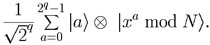
Notation: Here and in what follows |k>
in register L stands for |bq–1>
...
|b1>
|b0>, where
bq–1 ...
b1b0
is the binary representation of k, with a
similar convention for register R.
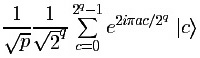
Step 3. We apply the Quantum Fourier Transform to register L.
This replaces each |a> by
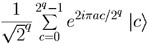 .
In Fig. 1, each column in the matrix corresponds to a standard
basis state for L, whereas the right-most column represents the
contents of register R; the state of
LR is
the superposition
.
In Fig. 1, each column in the matrix corresponds to a standard
basis state for L, whereas the right-most column represents the
contents of register R; the state of
LR is
the superposition
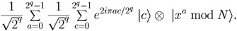
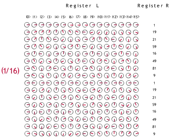
Fig. 1. Step 3 of the Shor Factorization Algorithm illustrated with
N = 85, x = 19 and q = 4.
Now the
LR register holds a superposition of 162
states, each weighted by 1/16. Reading from the top left, the first one is
e2 π 0·0/16|0>
|1>, i.e.
(e2 π 0·0/16
|0>
|0>
|0>
|0>)
(|0>
|0>
|0>
|0>
|0>
|0>
|1>);
the state corresponding to the last entry in the fourth row is
e2 π 3·15/16|15>
|59>, i.e.
(e2 π 3·15/16
|1>
|1>
|1>
|1>)
(|0>
|1>
|1>
|1>
|0>
|1>
|1>).
Before going to Step 4, let us note that the registers are set up
to carry out a Discrete Fourier Transform. But that algorithm would
require 2q multiplications for each of
2q rows: many too many operations. Shor's intuition
was that superposition and entanglement could be harnessed to do all
the work in a couple of steps, by first reading register R and
then reading register L.
Step 4. We examine register R. One of the values
will appear (they all have equal probability), and the others
will be lost. Suppose that value is
xα mod N. During the readout
the contents of register L collapse to those states which
were coupled with xα mod N
(compare Example 2 above).
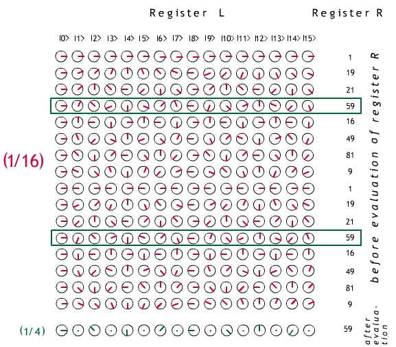
Fig. 2. Step 4 of Shor's Factorization Algorithm illustrated
with N = 85, x = 19 and q = 4. We suppose that
register R reads 59 (so α, as above, was 3 or 11).
Register L now only contains the
superposition of states which were entangled with |59>; these are
set off by the green boxes.
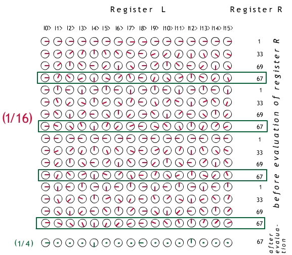
Fig. 3. Step 4 of Shor's Factorization Algorithm illustrated with
N = 85, x = 33 and q = 4; conventions as above.
We suppose that register R reads 67.
Step 5. We now read out register L. In the two examples we
have considered, the readout will be an exact multiple of
p = 2q/r. Repeating the experiment
with the same x a small number of times leads with very high
probability to a set of readouts whose only common divisor is p;
so r can be determined and the problem is solved.
These examples are untypically simple in that r (8 and 4 in
these two cases) was a power of 2, and therefore divided 2q
exactly.
In this simple situation, we can see how the readout takes us from
a superposition of states (in register R) with period
r to a superposition
of states (in register L) which have coefficient zero
unless they correspond to a
multiple of 2q/r. (Compare the examples;
this is the way the QFT detects frequency).
In fact, there will be exactly p = 2q/r values a
in the range [0,2q–1]
such that
xa =
xα mod N, and each of them
will contribute
to register L.
Since each of these a's is of the form α + kr,
k = 0, ..., p–1,
the factor of |c> is, up to a constant,
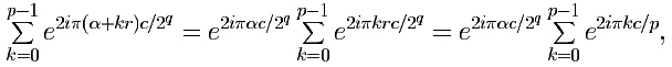
writing r = 2q/p for the
last equality.
The summation
cycles through a symmetric set of p-th roots of 1, and
is therefore zero, unless c is a multiple of p,
in which
case each term in the sum equals 1.
The general case requires a subtler analysis.
Now 2q/r is not an integer. The readout
in general cannot be an exact multiple of the frequency. But
using a long enough sample (here is where
the condition 2q > N2 comes into play
--to analyze 85 "realistically" we would have had to use
q = 13 and an 8192 x 8192 table of coefficients)
guarantees, with high probability, a useful approximation. Complete
details are in Shor's article referenced below.
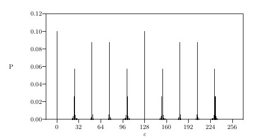
The calculated probabilities of a readout of c,
with r = 10 and 2q = 256. As Shor remarks,
the value r = 10 could occur when factoring 33 if x
were chosen to be 5, for example; 256 is chosen instead of
the required 211 to get a legible picture.
With high probability
the observed value of c is near an integral multiple
of 2q/r = 256/10. Image courtesy Peter
Shor.
References
General reference:
Peter W. Shor, Algorithms for Quantum Computation: In: Proceedings, 35th Annual Symposium on Foundations of Computer Science, Santa Fe, NM, November 20--22, 1994, IEEE Computer Society Press, pp. 124--134.
An
expanded version is available under the title
Polynomial-Time Algorithms for Prime Factorization
and Discrete Logarithms on a Quantum Computer, as
arXiv:quant-ph/9508027.
History of the Quantum Fourier Transform:
R. Cleve, A note on computing Fourier transforms by quantum programs,
unpublished, available as
postscript file
D. Coppersmith, An Approximate Fourier Transform Useful
in Quantum Factoring, IBM Research Report 07/12/94, available as
arXiv:quant-ph/0201067.
A. Ekert and R. Jozsa, Quantum computation and Shor's factoring
algorithm, Reviews of Modern Physics 68 (1996) 733-753