> with(plots):
with(DEtools):

First, lets define a few convenient abbreviations, so we needn't type our equations so verbosely

> Theta:=theta(t): V:=v(t):
Tdot:=diff(theta(t),t):
Vdot:=diff(v(t),t):
X:=x(t): Y:=y(t):
Xdot:=diff(x(t),t): Ydot:=diff(y(t),t):
S:=s(t): Sdot:=diff(s(t),t):

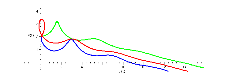
First, let's see what the flight of the glider looks like for a few different initial angles, but all with the same initial velocity. Note that here we are using the coordinates with a rescaled time variable.

> R:=.2;
DEplot([
Tdot= V*(V^2 - cos(Theta))/V,
Vdot= V*(-sin(Theta) -R*V^2),
Xdot= V*V*cos(Theta),
Ydot= V*V*sin(Theta)],
[theta,v,x,y],
t=0..20,v=0..2,theta=-Pi..Pi,
x=-1..15, y=-.5..4,
[[v(0)=2,theta(0)=Pi/4, x(0)=0,y(0)=2],
[v(0)=2,theta(0)=0, x(0)=0,y(0)=2],
[v(0)=2,theta(0)=-Pi/2,
x(0)=0,y(0)=2]],
scene=[X,Y],
stepsize=0.1,
linecolor=[red,green,blue],obsrange=false);

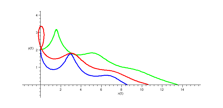
We would like the glider to stop flying once it hits the ground. One way to do this is to set the vector field to 0 if Y ever becomes negative. We can use piecewise to adjust the equations to account for this. Thus, the picture above becomes

> R:=.2;
DEplot([
Tdot= piecewise(Y>0,V*(V^2 - cos(Theta))/V,0),
Vdot= piecewise(Y>0,V*(-sin(Theta) -R*V^2),0),
Xdot= piecewise(Y>0,V*V*cos(Theta),0),
Ydot= piecewise(Y>0,V*V*sin(Theta),0)],
[theta,v,x,y],
t=0..20,v=0..2,theta=-Pi..Pi,
x=-1..15, y=-.5..4,
[[v(0)=2,theta(0)=Pi/4, x(0)=0,y(0)=2],
[v(0)=2,theta(0)=0, x(0)=0,y(0)=2],
[v(0)=2,theta(0)=-Pi/2,
x(0)=0,y(0)=2]],
scene=[X,Y],
stepsize=0.1,
linecolor=[red,green,blue],obsrange=false);

But, in fact, we want to know what the initial angle should be that will allow the glider to fly exactly 10 units. As a first step toward this, we can let maple create a procedure that gives us the location of the glider at any time. To do this, we use dsolve with the numeric option.

> fly:=dsolve( [
Tdot= piecewise(Y>0,V*(V^2 - cos(Theta))/V,0),
Vdot= piecewise(Y>0,V*(-sin(Theta) -R*V^2),0),
Xdot= piecewise(Y>0,V*V*cos(Theta),0),
Ydot= piecewise(Y>0,V*V*sin(Theta),0),
Sdot= piecewise(Y>0,V,0),
v(0)=2, theta(0)=0, x(0)=0, y(0)=2, s(0)=0],
[Theta,V,X,Y,S], type=numeric);

> fly(20);

From that, we can see that the middle solution (with initial angle 0) goes 13.458... before it hits the ground.
Since the initial conditions are part of the input to the procedure fly, to find out how the final position depends on the initial angle would mean calling dsolve again. This is tedious, so we write a little procedure to do it for us. It looks long, but it really is only dsolve followed by evaluating the solution at a given time.

> whereHit:= proc(theta0)
local x,y,v,t,s,theta,X,Y,V,S,R,
Theta,Xdot,Ydot,Vdot,Tdot,Sdot,v0,
sol,xhit,hittime;
R:=0.2;
v0:=2;

Theta:=theta(t): Tdot:=diff(theta(t),t):
V:=v(t): Vdot:=diff(v(t),t):
X:=x(t): Xdot:=diff(x(t),t):
Y:=y(t): Ydot:=diff(y(t),t):
S:=s(t): Sdot:=diff(s(t),t):

sol:=dsolve(
[Tdot= piecewise(Y>0,V*(V^2 - cos(Theta))/V,0),
Vdot= piecewise(Y>0,V*(-sin(Theta) -R*V^2),0),
Xdot= piecewise(Y>0,V*V*cos(Theta),0),
Ydot= piecewise(Y>0,V*V*sin(Theta),0),
Sdot= piecewise(Y>0,V,0),
x(0)=0, y(0)=2, v(0)=v0, theta(0)=theta0, s(0)=0],
[x(t),y(t),theta(t),v(t),s(t)],numeric);

hittime := 10;
while ((subs(sol(hittime)[3],y(t)) > 0)) do
hittime:= evalf(hittime + 10);
od;

xhit:=rhs(sol(hittime)[2]);
RETURN(xhit);
end:

Thus, we can get the same answer out of that routine a little simpler:

> whereHit(-Pi/2);
whereHit(0);
whereHit(Pi/4);

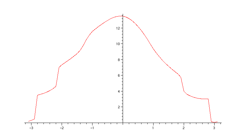
In fact, if we like, we can make a picture of how the final x value depends on the initial angle by graphing this function. Rather than plotting it directly,

it works better to just plot a sequence of values:

> plot([seq([z/10,whereHit(z/10)],z=-31..31)]);

A good graph would need some more points near -3 and +2, but this is good enough to let us know that we should concentrate near the angles .8 and .9, or between -1.4 and -1

> whereHit(.8);whereHit(.9);

We could just try values until we get what we want, but we can do this more efficiently using bisection, trapping the value we are looking for and narrowing in.

Here is a little maple procedure to do that for a general function.

> bisect:=proc(f,xlow_in,xhi_in,epsilon)
local xlow, xmid, xhi, flow, fmid, fhi;

xlow := xlow_in; flow:= f(xlow);
xhi := xhi_in; fhi := f(xhi);

if (sign(flow) = sign(fhi)) then
printf( `[%g,%g] and [%g,%g] dont bracket a zero\n`,
evalf(xlow), evalf(flow), evalf(xhi), evalf(fhi));
RETURN();
fi;


while( evalf(abs(xhi-xlow)) > evalf(epsilon)) do
xmid := evalf((xlow+xhi)/2);
fmid := f(xmid);
# print([xlow,flow], [xmid,fmid], [xhi,fhi]);
if (sign(fmid) = sign(fhi)) then
xhi := xmid;
fhi := fmid;
else
xlow:= xmid;
flow:= fmid;
fi;
od;
RETURN(xmid);
end:

> bisect(x->whereHit(x)-10.0, .8, .9, 0.00001);

> bisect(x->whereHit(x)-10.0, -1, -1.5, 0.00001);

So now, we can see them both flying merrily along, and landing right at 10.

> R:=.2;
DEplot([
Tdot= piecewise(Y>0,V*(V^2 - cos(Theta))/V,0),
Vdot= piecewise(Y>0,V*(-sin(Theta) -R*V^2),0),
Xdot= piecewise(Y>0,V*V*cos(Theta),0),
Ydot= piecewise(Y>0,V*V*sin(Theta),0)],
[theta,v,x,y],
t=0..20,v=0..2,theta=-Pi..Pi,
x=-1..11, y=0..3.5,
[[v(0)=2,theta(0)=.88642, x(0)=0,y(0)=2],
[v(0)=2,theta(0)=-1.2681, x(0)=0,y(0)=2]],
scene=[X,Y],
stepsize=0.1,
linecolor=[red,blue],obsrange=false);

>