Making an ellipse look like an ellipse

Suppose we have a dog in a yard. We know, or should know, that if we tie his leash down at one point and let him roam freely, he can reach any point which lies in a circle whose radius is the length of the leash, and the center is the point it is tied at.

Now, suppose we tie the leash at both ends, but allow the collar to slip along the rope. What set of points can the dog get to? Well, if we give the points the leash is attached at coordinates and and let the leash have length c, then the set of points which are accessible are given by the inequality

However, we need only consider the case of equality. Furthermore, using the distance formula, this becomes the set of points which satisfy

> dogEqn:= sqrt( (x-x[1])^2 + (y-y[1])^2) + sqrt( (x-x[2])^2 + (y-y[2])^2) = c:

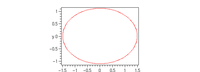
If you don't already know that this is an ellipse, we can use implicitplot to see that. Let us take our points to be (-1,0) and (1,0), and c=4. (The points are called the foci of the ellipse).

> myDogEqn := subs(x[1]=-1,y[1]=0,x[2]=1,y[2]=0,c=3,dogEqn);

> with(plots):

> implicitplot(myDogEqn, x=-2..2, y=-2..2, scaling=constrained,axes=boxed);

That surely looks like an ellipse to me. But how do we know it is an ellipse? From high school, I seem to remember (and maybe you do too) that the equation of an ellipse is of the form , and this doesn't look like that. So now we get to make it look like that.

But how? By algebraic messing around. This is, in fact, a little easier to do by hand on paper, but we will coerce maple into doing it anyway.

WARNING : most of this would be much easier to do on paper, with maple's assistance. but we are doing this for pedagogical reasons, and out of sheer meanness.

First, so that we can keep track of what is going on, let's replace the complicated stuff inside the square roots with something simpler. Then after we are done, we will put it back in.

> dogEqn1 := sqrt(e)+sqrt(f)=c;

We need to manipulate the left and right sides of the equation independantly, so lets give them names. The maple functions rhs and lhs give us the right and left sides of an equation:

> dogEqn1r := rhs(dogEqn1); dogEqn1l := lhs(dogEqn1);

Now we square both sides, in hopes that the square roots will go away (they won't).

> expand((dogEqn1l)^2) = (dogEqn1r)^2;

Doesn't look much better, huh? But notice that if we move the terms without a square root over to the other side, and then square both sides again, it will get rid of the roots.

> expand((dogEqn1l)^2-(e+f)) = (dogEqn1r)^2 - (e+f);

> expand(((dogEqn1l)^2-(e+f)))^2 = ((dogEqn1r)^2 - (e+f))^2;

The roots are gone. So that is what we want. Lets put everything on one side:

> dogFunc := expand( ((dogEqn1l)^2-(e+f))^2 - ((dogEqn1r)^2 - (e+f))^2);

Finally, we can substitute the real values of and back in.

> dogMess := expand(
subs(e=(x-x[1])^2 + (y-y[1])^2, f=(x-x[2])^2 + (y-y[2])^2, dogFunc));

Well, that looks awful. Lets see what we get when we put in our specific values of c, and , though:

> myDogMess := subs(x[1]=-1,y[1]=0,x[2]=1,y[2]=0,c=3,dogMess);

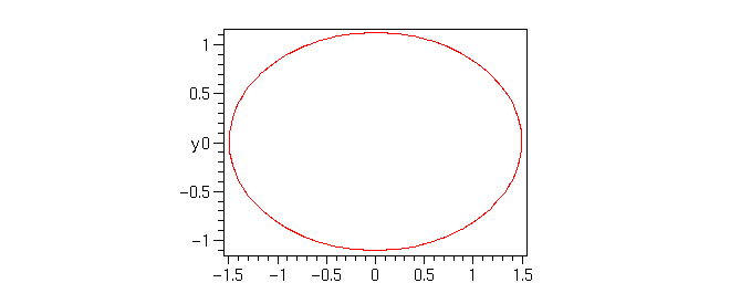
Not bad. Looks just like we'd expect an ellipse to look like. Let's plot it:

> implicitplot(myDogMess,x=-2..2, y=-2..2, scaling=constrained,axes=boxed);

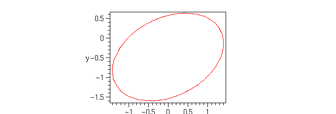
Yes, that is the same thing, and it is clearly the expected form. But, after that work, we have more: we have the general form of an ellips with foci at and with constant c. For example, a tilted ellipse:

> sort(subs(x[1]=-1,y[1]=-1,x[2]=1,y[2]=0,c=3,dogMess));

> implicitplot(",x=-2..2, y=-2..2, scaling=constrained,axes=boxed);

But let's see if we can neaten up this apparent mess a bit, collecting terms in x and y.

> collect(dogMess,[x,y],distributed);

Still pretty dreadful. Oh well. But we can make a general ellipse function out of it quite easily. Note that we will specify the two foci as A and B, so we need to have A= , and , so it looks like I made a mistake in the subs command. But I didn't.

> GenEllipse := (A,B,k) ->
simplify(subs(x[1]=A[1],y[1]=A[2], x[2]=B[1], y[2]=B[2], c=k, dogMess));

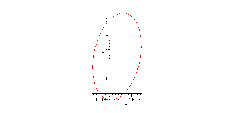
> GenEllipse([0,0],[1,5],6);

> implicitplot(GenEllipse([0,0],[1,5],6)=0,x=-2..3,y=-1..6,scaling=constrained);

The real question is: was it worth the trouble? (probably not).

>