We have already seen how to use maple to produce a graph of a function of one variable, such as
plot(sin(x),x=-2*Pi..2*Pi);
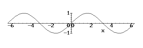
When Maple draws the graph of a function, basically what it does is pick a bunch of points equally spaced in the domain (typically 50), compute f(x), and connect the dots. Generally, Maple uses an "adaptive plotting method"; when the values of the function don't lie close to a straight line, Maple plots additional points in that region. This enables it to produce much better graphs. However, there is a limit to how well it can do in all cases.
For example, the function y=sin(1/x) does not have a limit as x nears 0; it wiggles more and more, oscillating between +1 and -1. Just asking Maple to draw its graph for -0.1 < x < 0.1 gives a rather unsatisfactory result:
plot(sin(1/x),x=-.1..0.1);
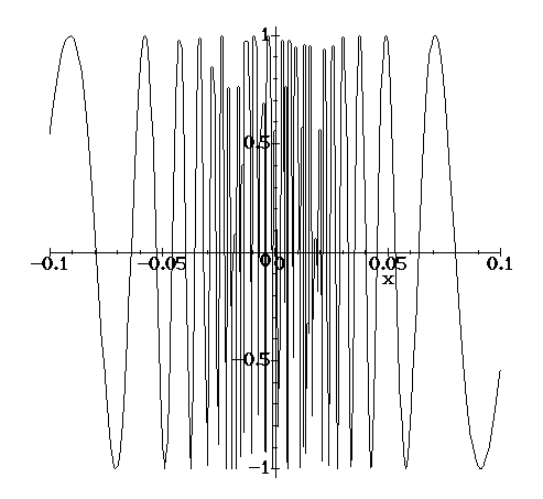
The real problem occurs when Maple samples the curve at points whose values just happen to lie near a straight line. It doesn't know any better, and gets fooled. We can make things a little better by asking Maple to sample more points initially (say, 1000 instead of just 50).
This does, however, waste a lot of computation on the regions where the graph behaves "nicely" ( for example, where |x| > 0.01).
plot(sin(1/x),x=-0.1..0.1,numpoints=10000);
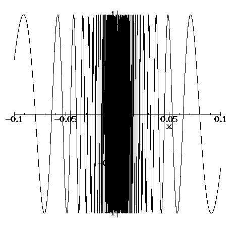
Note that this previous command took quite a long time to execute, however. Can you think of a "smarter" way to generate a good picture?