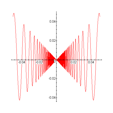
For the first problem, you had to figure out the meaning of the words "good" and "near". The main point was that the function has an envelope consisting of two parabolas, and it oscillates faster and faster as it approaches zero. One nice solution is the following:
plot(x^2 * sin(1/x), x=-.1..(.1), numpoints=2501);
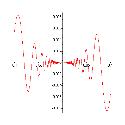
The second part is trickier because the function oscillates so much it is not even differentiable. A nice solution here was the following, although you can still see that the computer has a hard time showing all the oscillations near zero, so you just get a big dark area...
plot(x*sin(1/x),x=-.05..0.05, numpoints=1501);
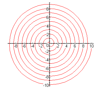
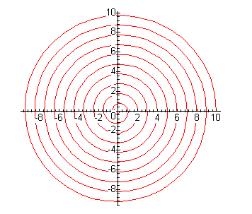
On to problem 2. Here the difficulty in the first part was to make the spirals go through the (positive) integers. There are a lot of ways of doing this, which all come down to noticing that the period of sine and cosine is 2*Pi, and so the angle should be 2*Pi*radius of the spiral:
plot([r*cos(2*Pi*r),r*sin(2*Pi*r), r=0..10],scaling=constrained);
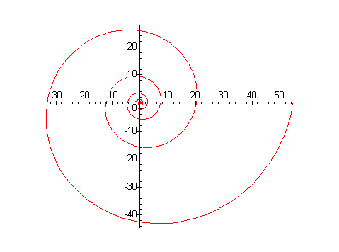
For part (b), most students noticed that all you have to do is to change the sign of either y or x to reverse the direction of the spiral. I'll show you how to do the problem in polar coordinates instead:
plot([r, -2*Pi*r, r=0..10], scaling=constrained, coords=polar);
Notice that my second spiral also goes through all the positive integers.(Most of yours go through the negative integers. Do you know why?)
The logarithmic spiral is one in which the angle changes logarithmically with the radius, or, the radius is the exponential of the angle. Here is one example, where I took out the axis so you can see the spiraling better. Notice that the angle in this case can take negative values, since the exponential is a positive function. Of course the spiral is 'infinite' at the origin, but we can only get good pictures of finite parts.
plot([exp(t), 2*Pi*t, t=-1.5..4],scaling=constrained, coords=polar, numpoints=500);
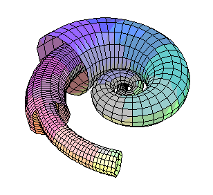
There were a considerable amount of choices to be made for the horn of plenty, and all of them looked pretty nice. Here's the maple command that produced the one in the handout:
with(plots):
tubeplot({[t*cos(5*ln(t)), t*sin(5*ln(t)), 0, t=exp(-500)..exp(1), radius=t/2],
          [t*cos(5*ln(t)), t*sin(5*ln(t)), 0, t=exp(.8)..exp(1.2), radius=t/4],
          [t*cos(5*ln(t)), t*sin(5*ln(t)), 0, t=exp(1)..exp(1.4) , radius=t/8]},
         axes=none, style=patch, scaling=constrained, tubepoints=15);
Now on to the tubeplot gallery. The first part was fairly straightforward.
with(plots):
tubeplot({[sin(t),cos(t),0], [sin(t)+1,0,cos(t)]},t=0..2*Pi,
         scaling=constrained,radius=.3);
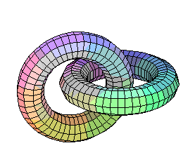
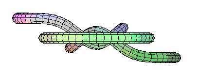
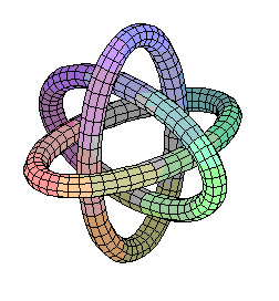
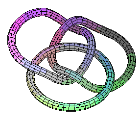
Now the rings were 'tricky', to say the least, but they were meant to be. There are a lot of acceptable ways of doing them. My favorite one is the following, which doesn't require any 'bumping', but of course you need to play around with strings or do something else to convince yourself that it is equivalent to the original picture in the handout.
tubeplot({[2*sin(t), cos(t), 0], [sin(t),0,2*cos(t)], [0,2*sin(t),cos(t)]},
          t=0..2*Pi, radius=.2, scaling=constrained);
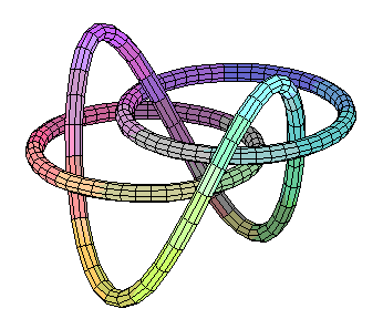
Here are some other pictures, most of which come from your solutions: The first one is what I tried to suggest to some people in class with the strings. It has two planar circles, one in the xz-plane and the other in the yz-plane, and the third one is a circle in the xy-plane with oscillating height function.
tubeplot({[sin(t), 0 , cos(t) -1.5], [0,sin(t), cos(t) +1.5],
          [.5*sin(t), .5*cos(t), 1.5*cos(2*t)]},
         t=0..2*Pi, radius=.1, scaling=constrained);
This one is fairly symmetric. Some students noticed that the bumps are sort of spread out at angle 2*Pi/3 apart. So with the height proportional to cos(3*t) things just work out.
tubeplot({[cos(t)+.5,sin(t),cos(3*t)],
          [cos(t)-.5,sin(t),cos(3*t)],
          [cos(t),sin(t)+.5,cos(3*t)]},
         t=0..2*Pi,scaling=constrained,radius=.1);
This following one has two circles planar and the third one weaving through. The height function is again a simple cosine, but it needed a little shifting to avoid intersections.
tubeplot({[cos(t),sin(t),0],
          [cos(t)-.85,sin(t),.25],
          [cos(t)-.25,sin(t)+.35,cos(2*t+2)]},
      t=0..2*Pi,radius=.08,scaling=constrained);
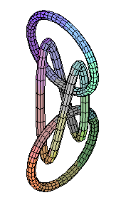
This one required some serious work, but it shows that one can actually do it just with bumps on one circle. It must have taken a while to work out, but the result is really nice.
tubeplot({[cos(t)-.5,sin(t)+.5,0],
          [cos(t),sin(t)-.4,2],
          [cos(t)+.5,sin(t)+.5,1-2*exp(-20*(t-2*Pi/3)^2)
                                +2*exp(-20*(t-Pi)^2)
                                -2*exp(-20*(t-(4*Pi/3))^2)
                                +2*exp(-20*(t-(5*Pi/3))^2)]},
         t=0..2*Pi,radius=.05,scaling=constrained,numpoints=100);
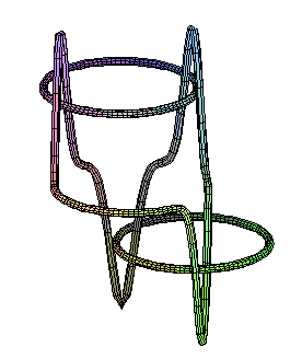
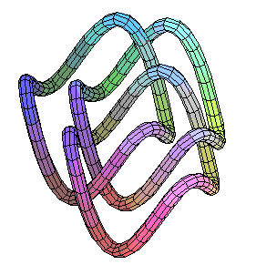
And here is the code Scott used to produce the picture in the handout:
tubeplot({ [2*sin(t)+1, 2*cos(t),     .75-exp( -(2*sin(t)+1)^2 ) ],
           [2*sin(t)-1, 2*cos(t),  - .75+exp( -(2*sin(t)-1)^2 ) ],
           [2*sin(t),  sqrt(3)+2*cos(t), 0 ]}, t=0..2*Pi, radius=0.2,
           axes=none, scaling=constrained);
And here's a side view. Scott's idea was to make the height of two of the circles dependent on the x-coordinate, and then bump one of them up and the other one down. I suggest you compare the picture with the formula again to see how it works.
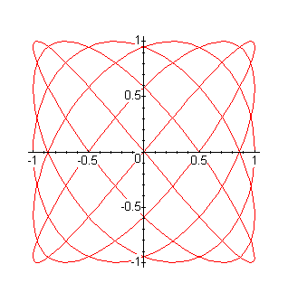
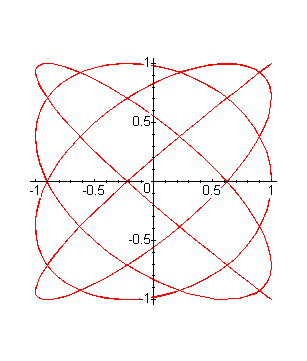
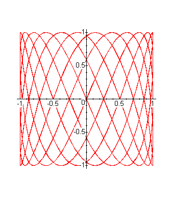
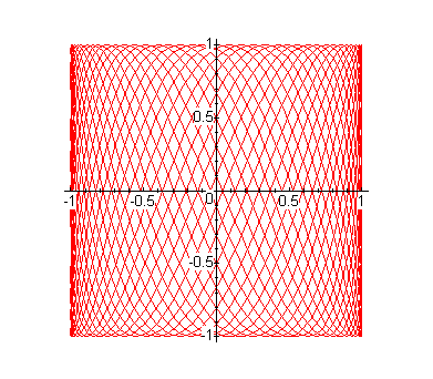
Well, now on to the last problem. As Scott pointed out in the handout, the point was for you to use maple to come up with conjectures about the curves of the form [cos(a*t), sin(b*t)] in the plane for various a and b. These are known as Lissajous figures, in case you want to read more about them somewhere in the math literature. Here are a few facts that experiments could have given you hints about, but the list is certainly not complete:
plot([cos(5*t), sin(6*t), t=0..2*Pi]);
plot([cos(8*t), sin(7*t), t=0..2*Pi]);
plot([cos(15*t), sin(36*t), t=0..2*Pi]);
plot([cos(15*t), sin(37*t), t=0..2*Pi]);
There are other things one can say, and I encourage you to either play around some more or find a book that talks about these things.