Easy reading on topology of real plane algebraic curves
This is a shortened version of introduction to book “Topological Properties of Real Plane Algebraic Curves” by V.M.Kharlamov, V.A.Rokhlin and O.Y.Viro. This book is still under preparation. We have just taken away all the references to the main body of the book.
Here we would like to offer several variations on the central themes of topology of real plane algebraic curves. We do this only to give a first impression of the subject. This is not a formal introduction to the subject; rather, it should be considered a sort of pure advertisement. Here, more than in a textbook, we will opt for elementary, specific considerations instead of generality.
We were encouraged to write in this way by the fortunate features peculiar to our subject: elementary formulations and a rare combination of simple, natural problems and surprising, beautiful solutions. Unfortunately, these features are easily overlooked in the environment of a traditional exposition.
1 Curves under Consideration
Our main subject is the topological properties of nonsingular real projective plane algebraic curves. These curves are nice, elementary classical objects. However, as a prelude, we will restrict ourselves to even more elementary objects, which are suitable even in the scope of high school mathematics but still suffice to demonstrate the beauty of the subject.
Namely, we consider curves on the affine plane $\mathbb{R}^{2}$ defined by equations of the form $f(x,y)=0$, where $f$ is a real polynomial in two variables. We impose two further conditions on $f$. First, we require the curves to be nonsingular. This means that at no point of the curve do the first partial derivatives of $f$ vanish simultaneously.
Second, we require the homogeneous part of the highest degree of $f$ to be positive or negative definite, i.e., to have no nontrivial zero. The second condition implies compactness of the curve; it can be fulfilled only if the degree of the curve is even.
Here we want, on the one hand, to stay in the affine plane, but, on the other hand, to avoid the usual complications related to branches tending to infinity. In particular, we want to prevent the topology of a curve from being unstable under small perturbations.
Throughout this text, by a curve we mean a curve of degree $m=2k$ satisfying the two conditions stated above.
Under these two conditions, each connected component of the curve is a topological circle smoothly embedded in $\mathbb{R}^{2}$; the number of the circles is finite. Traditionally, the components are called ovals even though they may be nonconvex.
The topology of such a curve is just the number of its ovals and their mutual position in the plane. In other words, the topology is determined by the following obvious partial order in the set of ovals: an oval $C$ is greater than an oval $C^{\prime}$ if $C$ envelops $C^{\prime}$; if $C$ and $C^{\prime}$ bound disjoint disks in $\mathbb{R}^{2}$, then they are not comparable.
There is no restrictions on the topology of a real algebraic curve as long as no condition on its equation is imposed. Moreover, any finite collection of disjoint smoothly embedded circles can be approximated with any precision by a real algebraic curve.
2 Curves of Low Degrees
The smaller the degree of curves, the simpler they are topologically. The first case, degree 2, is the simplest one and is familiar to anyone who has studied the classical theory of conics. A curve of degree 2 (satisfying our conditions) either is an ellipse or has no real points.
The case of degree 4 is also simple. To classify quartics (curves of degree 4), first note that the number of ovals of a quartic is at most 4. Indeed, if a curve of degree 4 had five (or more) ovals then, taking a point in each of these five ovals and tracing a conic through the five selected points, one would get $\geq 10$ intersection points; this would contradict the Bezout theorem, which asserts that this number is bounded by $8=2\cdot 4$.
The mutual position of the ovals of a quartic cannot be complicated either: if their number is strictly greater than 2, then none of the ovals lies inside another one. The proof is again provided by the Bezout theorem: if there were an oval lying inside another one, then, tracing a line through a point inside the inner oval and a point on a third oval, one would get at least six common points of the curve and the line, which is impossible.
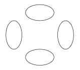
Therefore, the ovals of a quartic can have only one of the mutual positions shown in Figure 1.
 |
 |
 |
| $\langle 4\rangle$ | $\langle 3\rangle$ | $\langle 2\rangle$ |
 |
 |
no ovals |
| $\langle 1\langle1\rangle\rangle$ | $\langle 1\rangle$ | $\langle 0\rangle$ |
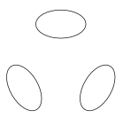
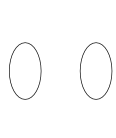
There exist curves that have all of these schemes of mutual position of ovals. An empty curve is defined by the equation $x^{4}+y^{4}+1=0$. To construct the nonempty curves, one can perturb the union of two ellipses by introducing a small additional term into the equation, see Figure 2. Note that, unlike most drawings below, Figure 2 represents the true shape of the curves.


The next case, degree 6, is the first really difficult one. Here the number of ovals is $\leq 11$ (this is a special case of a general bound on the number of ovals for a curve of a given degree called the Harnack inequality).
Still, the mutual position of ovals cannot be very complicated: unless the number of ovals is 3, at most one of them is not empty (i.e., envelops ovals). This follows from the Bezout theorem, like the similar statement on quartics above. If a curve has three ovals, they can be placed in a concentric fashion. All the other nonempty curves of degree 6 are organized as follows: several, say $\alpha+1$, ovals lie outside each other and one of them encircles several, say $\beta$, other ovals which are placed outside each other. In the bracket notation for the mutual position of ovals such a curve is denoted by $\langle\alpha\amalg 1\langle\beta\rangle\rangle$.
In Table 1 we list all schemes11This book is so elementary that we allow ourselves to use the word scheme in its ordinary sense not as it is understood in modern algebraic geometry. of curves of degree 6.
| $\displaystyle\ \ \langle 9\amalg 1\langle 1\rangle\rangle\ \ \phantom{% \langle 9\amalg 1\langle 1\rangle\rangle\ \ \langle 9\amalg 1\langle 1% \rangle\rangle\ \ \langle 9\amalg 1\langle 1\rangle\rangle}\ \ \langle 5% \amalg 1\langle 5\rangle\rangle\ \ \phantom{\langle 9\amalg 1\langle 1% \rangle\rangle\ \ \langle 9\amalg 1\langle 1\rangle\rangle\ \ \langle 9% \amalg 1\langle 1\rangle\rangle}\ \ \langle 1\amalg 1\langle 9\rangle\rangle$ | ||
| $\displaystyle\langle 10\rangle\ \ \langle 8\amalg 1\langle 1\rangle\rangle% \ \ \phantom{\langle 9\amalg 1\langle 1\rangle\rangle\ \ \langle 9\amalg 1% \langle 1\rangle\rangle}\ \ \langle 5\amalg 1\langle 4\rangle\rangle\ \ % \langle 4\amalg 1\langle 5\rangle\rangle\ \ \phantom{\langle 9\amalg 1% \langle 1\rangle\rangle\ \ \langle 9\amalg 1\langle 1\rangle\rangle}\ \ % \langle 1\amalg 1\langle 8\rangle\rangle\ \ \langle 1\langle 9\rangle\rangle$ | ||
| $\displaystyle\phantom{\langle 10\rangle}\langle 9\rangle\ \ \langle 7\amalg 1% \langle 1\rangle\rangle\ \ \langle 6\amalg 1\langle 2\rangle\rangle\ \ % \langle 5\amalg 1\langle 3\rangle\rangle\ \ \langle 4\amalg 1\langle 4% \rangle\rangle\ \ \langle 3\amalg 1\langle 5\rangle\rangle\ \ \langle 2% \amalg 1\langle 6\rangle\rangle\ \ \langle 1\amalg 1\langle 7\rangle\rangle% \ \ \langle 1\langle 8\rangle\rangle$ | ||
| $\displaystyle\phantom{\langle 10\rangle}\langle 8\rangle\ \ \langle 6\amalg 1% \langle 1\rangle\rangle\ \ \langle 5\amalg 1\langle 2\rangle\rangle\ \ % \langle 4\amalg 1\langle 3\rangle\rangle\ \ \langle 3\amalg 1\langle 4% \rangle\rangle\ \ \langle 2\amalg 1\langle 5\rangle\rangle\ \ \langle 1% \amalg 1\langle 6\rangle\rangle\ \ \langle 1\langle 7\rangle\rangle$ | ||
| $\displaystyle\phantom{\langle 10\rangle}\langle 7\rangle\ \ \langle 5\amalg 1% \langle 1\rangle\rangle\ \ \langle 4\amalg 1\langle 2\rangle\rangle\ \ % \langle 3\amalg 1\langle 3\rangle\rangle\ \ \langle 2\amalg 1\langle 4% \rangle\rangle\ \ \langle 1\amalg 1\langle 5\rangle\rangle\ \ \langle 1% \langle 6\rangle\rangle$ | ||
| $\displaystyle\phantom{\langle 10\rangle}\langle 6\rangle\ \ \langle 4\amalg 1% \langle 1\rangle\rangle\ \ \langle 3\amalg 1\langle 2\rangle\rangle\ \ % \langle 2\amalg 1\langle 3\rangle\rangle\ \ \langle 1\amalg 1\langle 4% \rangle\rangle\ \ \langle 1\langle 5\rangle\rangle$ | ||
| $\displaystyle\phantom{\langle 10\rangle}\langle 5\rangle\ \ \langle 3\amalg 1% \langle 1\rangle\rangle\ \ \langle 2\amalg 1\langle 2\rangle\rangle\ \ % \langle 1\amalg 1\langle 3\rangle\rangle\ \ \langle 1\langle 4\rangle\rangle$ | ||
| $\displaystyle\phantom{\langle 10\rangle}\langle 4\rangle\ \ \langle 2\amalg 1% \langle 1\rangle\rangle\ \ \langle 1\amalg 1\langle 2\rangle\rangle\ \ % \langle 1\langle 3\rangle\rangle$ | ||
| $\displaystyle\phantom{\langle 1\langle 1\langle 1\rangle\rangle\rangle}\qquad% \langle 3\rangle\ \ \langle 1\amalg 1\langle 1\rangle\rangle\ \ \langle 1% \langle 2\rangle\rangle\qquad\langle 1\langle 1\langle 1\rangle\rangle\rangle$ | ||
| $\displaystyle\langle 2\rangle\ \ \langle 1\langle 1\rangle\rangle$ | ||
| $\displaystyle\langle 1\rangle$ | ||
| $\displaystyle\langle 0\rangle$ |
The shape of this list seems difficult to foresee. However, the shape is not artificial. It is determined by the nature of things. In the table each row is occupied by schemes with the same number of ovals. One can easily find an explanation for the placement of the schemes within each row as well.
This book contains, among other things, a proof of this classification. This particular result has a dramatic history in which a number of famous mathematicians have participated. Our advertisement would be incomplete without at least a brief account of these events. However, we want to present the subject first, postponing the history to the end of the Introduction.
3 Prohibitions and Constructions
To classify the curves of a given degree it is natural to work in two directions: first, to look for restrictions which the algebraic nature of a curve imposes on its topology; and, second, to prove that any mutual position of ovals which satisfies these restrictions is realized.
The prohibitions and constructions (as we shall call the results in the first and second direction, respectively) cannot be considered separately. Rather, they are two complementary ways of answering the same question: What topology is possible for a real algebraic curve of a given degree? For example, the list of schemes for curves of degree 8 is not yet completely known. In particular, there are 6 $M$-schemes whose inclusion in the list is still undertermined.
4 Prohibition Inequalities and Prohibition Congruences
The complicated shape of the table of curves of degree 6 stems from a collection of four restrictions on the topology of these curves. Two of them have been formulated above: the restriction on the number of ovals enveloping other ovals and the Harnack inequality.
The Harnack inequality was formulated in the preceding Section only for curves of degree 6. Here is the general statement.
4.A
Harnack Inequality. The number of components of a curve of degree $m$ is at most $\frac{1}{2}(m-1)(m-2)+1$.
This is a typical prohibition inequality. To formulate other restrictions of this kind we need other numerical characteristics of a curve. Each oval of a curve lies inside a certain number of other ovals (of course, this number may be zero). An oval is said to be even if this number is even, otherwise it is said to be odd. The number of even ovals is denoted by $p$, the number of odd ovals by $n$.
As is well known, two integers may be related not only by an inequality, but also by a congruence.
4.B
Gudkov-Rokhlin Congruence. For any curve of degree $m=2k$ with the maximal number of ovals (equal to $\frac{1}{2}(m-1)(m-2)+1$),
| $p-n\equiv k^{2}\mod 8.$ |
The Gudkov-Rokhlin congruence explains why the top line of the table of curves of degree 6 contains only three schemes.
4.C
Gudkov-Krakhnov-Kharlamov Congruence. For any curve of degree $m=2k$ with the number of ovals equal to $\frac{1}{2}(m-1)(m-2)$ (that is, the maximal number minus 1),
| $p-n\equiv k^{2}\pm 1\mod 8.$ |
The Gudkov-Krakhnov-Kharlamov congruence explains the lacunae in the second line of the table.
Technically, most restrictions on the topology of a curve (both inequalities and congruences) belong to topology. Theorems 4.B and 4.C are related to some congruences discovered in arithmetic and differential topology in the middle of the XX century.
5 Ovals Emerging from a Singular Point
Although we want to construct nonsingular curves, the construction often starts with a singular one. For example, to construct the curves in the top line of the table of curves of degree 6, one can start from three ellipses tangent to each other at two points. See Figure 3. The union of these ellipses is defined by the product of the equations of the ellipses. Thus it is a curve of degree 6. It has two singular points. At each point there are three branches tangent to each other in the simplest way (i.e. quadratically).

We perturb this curve by perturbing its equation. A small perturbation does not change the topology of a curve far from its singular points, but near a singular point the changes may be drastic. Our goal is to choose the perturbation in a special way, taking into account the change of topology near the singular points.
| $\alpha=$ | 4 | 0 | 3 | 0 | 2 | 1 | 0 | 1 | 0 | 0 |
|---|---|---|---|---|---|---|---|---|---|---|
| $\beta=$ | 0 | 4 | 0 | 3 | 0 | 1 | 2 | 0 | 1 | 0 |
| $\gamma=$ | 3 | 2 | 1 | 0 | 0 |
|---|---|---|---|---|---|
| $\delta=$ | 0 | 0 | 0 | 1 | 0 |
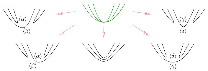
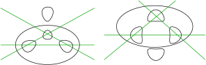
What piece of curve can emerge from a singular point? In the case under consideration the answer is shown in Figure 4. Up to four new ovals may appear. If their number is exactly 4, then they may be positioned only in two ways.
Figure 4 resembles the table of curves of degree 6, but it is a bit smaller. The problem of classifying the pictures emerging from a singular point is similar to that of classifying the position of ovals of nonsingular curves of a given degree. In particular, its solution also involves prohibitions and constructions. However, passing from curves of degree 6 to perturbations of a point of quadratic contact of three branches reduces the complexity of the problem.
Furthermore it turns out that it is possible to operate at two singular points simultaneously and independently. In particular, one can perturb the union of three ellipses shown in Figure 3 in such a way that at each of the singular points four new small ovals emerge, positioned independently in one of two possible ways. This is shown in Figure 5. This gives all the curves in the top line of the table of curves of degree 6.

6 Complex Vision of Real Curves
A real algebraic curve is something more than just the set of its real points $\{(x,y)\in\mathbb{R}^{2}\,:\,f(x,y)=0\}$. It also has imaginary points, i.e., points of the complex plane $\mathbb{C}^{2}$ satisfying the same equation $f(x,y)=0$. When studying the topology of the set of real points of a curve, it is very useful to keep in mind the set of all its complex points.
Proofs of most prohibitions of the prohibitions stated in Section 5 demand consideration of the set of complex points. However, it is impossible to confine the complex domain to the proofs. Sooner or later, it shows up in the formulations. Without a complex vision many phenomena in the real domain are impossible to describe.
Topologically the set of complex points of a real curve is a surface, which may have a finite number of (imaginary) singular points. By a perturbation of the equation one can make the set of complex points topologically standard: homeomorphic to a sphere with $\frac{1}{2}(m-1)(m-2)$ handles punctured at $m$ points. Since a perturbation does not change the topology of the set of real points, we assume that such a perturbation has been done.
As a result, the set of real points of a curve can lie in the set of its complex points in two ways. It may happen that the former divides the latter into two connected halves, which are interchanged by the complex conjugation involution $\mathbb{C}^{2}\to\mathbb{C}^{2}:(z,w)\mapsto(\bar{z},\bar{w})$. In this case the curve is said to be of type I, or dividing. Otherwise, the complement of the set of real points of the curve in the set of its complex points is connected. Then the curve is said to be of type II, or nondividing.
An ellipse is of type I: its set of complex points is homeomorphic to $S^{1}\times\mathbb{R},$ the real part lies in it as the fiber $S^{1}\times 0$, and the conjugation acts as the symmetry $(z,t)\mapsto(z,-t)$. A curve of degree 2 without real points is of type II: the empty set cannot divide anything.
A curve of degree $m$ with $\frac{1}{2}(m-1)(m-2)+1$ ovals (recall that this is the maximal number of ovals for degree $m$) is of type I, because that many ovals necessarily divide a sphere with $\frac{1}{2}(m-1)(m-2)$ handles. In fact a similar argument proves the Harnack inequality: a sphere with $\frac{1}{2}(m-1)(m-2)$ handles cannot be divided into less than three connected pieces by a collection of $>\frac{1}{2}(m-1)(m-2)+1$ disjoint embedded circles. Furthermore, the number of ovals of a dividing curve of degree $m=2k$ is congruent to $k$ modulo 2. This follows from a well-known theorem according to which the number of connected components of a compact oriented surface is congruent modulo 2 to the Euler characteristic of the surface. Indeed, a dividing curve bounds a half of its complexification, whose Euler characteristic is the half of the Euler characteristic of the whole complexification, that is $$\frac{1}{2}(2-2\frac{(m-1)(m-2)}{2})=\frac{1}{2}(3m-m^{2})=3k-2k^{2}\equiv k\mod 2$$.
As we shall see, in many respects curves of type I are more interesting than curves of type II. First, curves of type I bear an additional structure coming from the complex domain.
If the real part of a curve divides its complexification, then each of the halves has the canonical orientation defined by the complex structure and defines an orientation on the common boundary of the halves, which is the set of real points. Thus the set of real points receives two orientations. It is easy to see that these orientations are opposite to each other. They are called the complex orientations of the curve.
A collection of $n$ ovals can be oriented in $2^{n}$ distinct ways. Therefore, if the number of ovals is greater than one, the pair of complex orientations is a new structure on the real part of the curve which comes from the complex domain. If one insists on the purely real viewpoint, ignoring all complex phenomena, the complex orientations look mysterious: a choice of orientation of one of the ovals determines the orientations of all the other ovals.
The scheme of the mutual position of ovals enhanced by the type of the curve and, in the case of type I, by a description of the complex orientations is called the complex scheme of a real curve. The bare scheme of the mutual position of the ovals is called its real scheme.
Complex schemes are subject to numerous topological restrictions, similar to restrictions on real schemes. For example, as was shown above, a curve with the maximal number of ovals is of type I, while a curve without real points is of type II.
To formulate a restriction on the complex orientations, let us introduce the numerical characteristics of an oriented curve on the plane. Denote the number of ovals with counterclockwise orientation by $\Lambda^{+}$ and the number of ovals with clockwise orientation by $\Lambda^{-}$. A pair of ovals in which one envelops the other one is called an injective pair. An injective pair of oriented ovals is said to be negative if the ovals are both oriented either clockwise or counterclockwise. Otherwise it is said to be positive. See Figure 6.
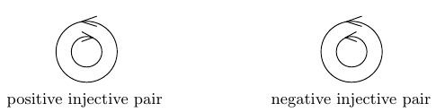
The number of positive injective pairs of ovals is denoted by $\Pi^{+}$, the number of negative injective pairs by $\Pi^{-}$.
6.A
Rokhlin Complex Orientation Formula. For any curve of type I and degree $m=2k$ with $l$ ovals,
| $2(\Pi^{+}-\Pi^{-})=l-k^{2}.$ |
This theorem is a strong restriction on the complex orientation and type. In particular, it explains why in degree 4 the real schemes $\langle 3\rangle$, $\langle 2\rangle$, $\langle 1\rangle$ are of type II, and it determines the complex orientations for $\langle 1\langle 1\rangle\rangle$.
Theorem 6.A implies even some restrictions on real schemes. For example, it implies that a curve of degree 6 cannot consist of 11 ovals lying outside each other (this follows from the Gudkov-Rokhlin congruence, too). Indeed, since 11 is the maximal number of ovals for a curve of degree 6, the curve should be of type I. Therefore it must have an orientation satisfying the Rokhlin complex orientation formula. The left-hand side of this formula is 0, since no pair of ovals is injective. The right-hand side is $11-3^{2}=2$. Thus, the formula cannot hold true.
7 Mutual Position of a Pair of Dividing Curves
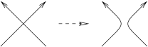
The complex domain allows one to see new features of the mutual position of a pair of real algebraic curves and formulate new restrictions on it. Consider two curves of type I. Assume that they intersect each other transversely. Choose a complex orientation (one of the two) on each of them. This choice is equivalent to a choice of one of the halves of the complexification. At each common point of the real parts of the curves one can smoothen their union according to the orientations, as shown in Figure 7. The smoothened curve inherits an orientation.
7.A
Complex Orientation Formula for a Pair of Curves. For any pair of curves of type I and degrees $m_{1}$ and $m_{2}$ which have $c$ common real points and intersect transversely, there exists an even number $\sigma$ such that $0\leq\sigma\leq m_{1}m_{2}-c$ and
| $\sigma=2(\Pi^{+}-\Pi^{-})-l+\frac{(m_{1}+m_{2})^{2}}{4},$ | (1) |
where $l$ and $\Pi^{\pm}$ are, respectively, the number of ovals and the number of positive or negative injective pairs of ovals of the smoothing of the union of the real parts of the curves in accordance with some complex orientations.
7.B
Corollary: Affine Complex Orientation Inequality.For any curve of type I and degree $m=2k$,
| $|\Lambda^{+}-\Lambda^{-}|\leq k.$ |
Proof. the pair consisting of the curve and a circle which envelops the curve. Apply Theorem 7.A to this pair, the circle oriented clockwise. The curve does not meet the circle. Hence the numbers $\Pi^{\pm}$ in (1) are equal to $\Pi^{\pm}+\Lambda^{\pm}$ for the original curve, and (1) turns into
| $\sigma=2(\Pi^{+}-\Pi^{-}+\Lambda^{+}-\Lambda^{-})-l-1+(k+1)^{2}.$ |
On the other hand, by the Rokhlin complex orientation formula 6.A, $2(\Pi^{+}-\Pi^{-})=l-k^{2}$. Therefore, $\sigma=2(\Lambda^{+}-\Lambda^{-})+2k$. By 7.A, $0\leq\sigma\leq 4k$. Hence $|\Lambda^{+}-\Lambda^{-}|\leq k.$ $\Box$
7.C
Corollary. For any curve of type I and degree $m=2k$, the number of ovals is at least $k$. $\Box$
7.D
Corollary. In a complex orientation of a curve of degree 4 consisting of four ovals at least one oval is oriented clockwise and at least one counterclockwise. $\Box$
The orientations not prohibited by 7.D are realized as complex orientations: there are curves of degree 4 with the complex orientations shown in Figure 8.

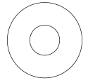
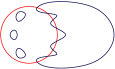
One can imagine a mutual position of two curves which admits no orientation satisfying 7.A. Such mutual positions are prohibited. For example, a curve of degree 4 with four ovals cannot be placed with respect to a circle as shown in Figure 9.
The number $\sigma$ in Theorem 7.A has the following geometric meaning. Without loss of generality we may assume that the complexifications of the curves are also transversal: otherwise we can slightly perturb one of the curves while preserving the mutual position of their real parts. For the same reason we may assume that the curves have no common imaginary asymptotic direction. Under these assumptions $\sigma$ is the total number of imaginary intersection points of the halves of the curves corresponding to the selected complex orientations with the halves corresponding to the opposite orientations.
This interpretation allows one to find or estimate the number of common points of the halves of the curves. Consider an example. Two ellipses positioned in the plane outside each other and having no common imaginary asymptotes intersect each other in the complex domain in such a way that each half of one of them meets each half of the other in one point. If the ellipses form an injective pair, then their halves corresponding to orientations making this pair positive are disjoint. The halves which correspond to orientations making this pair negative intersect each other in two imaginary points or have a common imaginary asymptotic direction.
8 Rigid Isotopy
The two conditions introduced into the definition of a curve in Section 1 above imply that a small perturbation of a curve does not change its topology. Thus, the topology is preserved under any continuous change of the equation during which the curve still satisfies the conditions of Section 1. This suggests the following question: given two curves of the same degree, when is it possible to deform one of them to the other one continuously, i.e., when they belong to the same component of the space of curves? A path in this space is called a rigid isotopy. Curves are said to be rigidly isotopic if there exists a rigid isotopy connecting them.
Of course, the mutual positions of the ovals of two rigidly isotopic curves are the same. However, this obvious necessary condition is far from being sufficient.
Indeed, under a rigid isotopy not only the real scheme, but also the complex scheme,22Recall that the type and the complex scheme of a curve were defined in 6 only for curves whose complexification is topologically standard. So, the natural, and correct, way to understand this assertion is to compare the whole space of curves with its subspace constituted by curves with topologically standard complexification. They turn out to have the same decomposition into connected components: if two curves with topologically standard complexifications are rigidly isotopic they can be connected by a rigid isotopy constituted by curves with topologically standard complexification. is preserved. Therefore the curves of degree 4 shown in Figure 8 are not rigidly isotopic.
It may happen that the complex schemes of curves of the same degree are the same but that the curves are still not rigidly isotopic. The simplest example is the pair of curves of degree 6 shown in Figure 10.
These curves are of type II (the Rokhlin complex orientation formula implies that they cannot be of type I). The obstruction to rigid isotopy is provided by the Bezout theorem. A line intersecting two internal ovals meets the curve in six points (two on each of these internal ovals and two on the oval encircling them). The external oval cannot move through such a line, since the total number of intersection points is at most 6 by the Bezout theorem. In the curves considered the external ovals occupy different positions with respect to the three lines connecting the pairs of internal ovals.
Fragments of History
9 Concise History of Degree 6
As far as we know, no specific results concerning the topology of nonsingular real plane curves of degree $\geq 6$ were obtained until 1876. That year marks the beginning of the topological study of real algebraic curves. Prior to 1876 topological properties were not treated separately from other geometric properties, which are more subtle and could keep geometers busy with curves of lower degrees.
In 1876 A. Harnack published a paper [2] giving a sharp upper bound for the number of components of a curve of a given degree. Harnack proved Theorem 4.A and for any natural $m$ constructed a nonsingular real projective curve of degree $m$ with $\frac{1}{2}(m-1)(m-2)+1$ components, which shows that this theorem cannot be improved without introducing new ingredients. Strictly speaking, all of these results are stated in [2] for projective curves, but they imply the same statements for the curves introduced in Section 1 and, moreover, the proofs can be adjusted. For curves of degree 6 Harnack’s results mean that the number of ovals is at most 11 and there exists a curve with 11 ovals. The curves of degree 6 with 11 ovals constructed by Harnack have the scheme $\langle 9\amalg 1\langle 1\rangle\rangle$.
It was D. Hilbert who made the first attempt to study the topology of nonsingular real plane algebraic curves systematically. The first difficult special problems that he encountered involved curves of degree 6.
Hilbert suggested that from the topological viewpoint, among the curves of a given degree $m$ the most interesting are curves with the maximal number $\frac{1}{2}(m-1)(m-2)+1$ of components. Hilbert’s guess was strongly confirmed by the whole subsequent development of the field. Now, following I. Petrovsky, these curves are called M-curves. In degree 6, M-curves are curves with 11 components.
Hilbert succeeded in constructing an M-curve of degree 6 with a scheme different from the one realized by Harnack. However, he realized only one new scheme, namely $\langle 1\amalg 1\langle 9\rangle\rangle$. He conjectured that these are the only schemes realizable by M-curves of degree 6 and for a while he believed that he had a (long) proof of this conjecture. Even though it was false (it was disproved in 1969 by D.Gudkov, who constructed a curve with the scheme $\langle 5\amalg 1\langle 5\rangle\rangle$), this conjecture caught the essence of what in the thirties and the seventies would become the core of the theory: prohibition inequalities and prohibition congruences.
In fact, Hilbert invented a method which allows one to answer all of the questions concerning the topology of curves of degree 6. It involves a detailed analysis of the singular curves which can be obtained from a given nonsingular one. The method required sophisticated fragments of singularity theory, which had not yet been elaborated at the time of Hilbert.
This project was realized in its entirety only in the sixties, by D. A. Gudkov. It was Gudkov who obtained the table of schemes shown above. However, let us maintain our chronological order.
Hilbert attracted attention of the world mathematical community to the topology of real algebraic varieties by including into his famous problem list [3], as the sixteenth problem, a collection of selected special problems on topology of real algebraic curves and surfaces, like the problem concerning possible mutual positions of the ovals of a plane $M$-curve of degree 6.
The choice of the number sixteen for this problem is intriguing. That number plays a very special role in the topology of real algebraic varieties. Most of the prohibition congruences, including 4.B and 4.C sutiably reformulated, were proved as congruences modulo sixteen. However, it is difficult to believe that Hilbert was aware of phenomena that would not be discovered until some seventy years later. Nonetheless, that was the number chosen by Hilbert.
10 Insights and Conjectures
The next story we have to tell concerns a work which contains no results on curves of degree 6 and, in a sense, almost no results at all. In 1906, V. Ragsdale [9] made a remarkable attempt to analyze Harnack’s and Hilbert’s constructions in order to devise new restrictions on the topology of curves. To a great extent the success of her analysis was due to the right choice of parameters of a scheme. Ragsdale suggested that one distinguish even and odd ovals. She provided good reasons why special attention should be paid to $p$ and $n$: a curve of even degree divides the plane into two pieces with common boundary (which is the curve itself, of course), and all the Betti numbers of the halves can be expressed in terms of $p$ and $n$. Ragsdale also singled out the difference $p-n$, motivating this by the fact that it is the Euler characteristic33At that time the terminology was different, and she wrote about Kronecker’s characteristics and their geometrical interpretation given by Dyck. of one of the halves of the plane. (It is amazing to find such considerations in a paper dated 1906!)
By analyzing the constructions, Ragsdale [9] made the following observations.
10.A
For any Harnack $M$-curve of even degree $m=2k$,
| $p=\frac{3k(k-1)}{2}+1,\qquad n=\frac{(k-1)(k-2)}{2}.$ |
For any Hilbert $M$-curve of even degree $m=2k$,
| $\displaystyle\frac{(k-1)(k-2)}{2}+1\leq p\leq\frac{3k(k-1)}{2}+1,$ | ||
| $\displaystyle\frac{(k-1)(k-2)}{2}\leq n\leq\frac{3k(k-1)}{2}.$ |
She wrote: “As curves of higher order are investigated a most interesting law governing the arrangement of the ovals present itself so persistently, and in curves of such widely different types, as to give strong reasons for belief in the existence of a general theorem.”
The main formulation suggested by Ragsdale can be interpreted in our terms as follows.
10.B
For any $M$-curve of degree $m=2k$,
| $n\geq{(k-1)(k-2)\over 2},\,\text{ or, equivalently,}\quad p\leq{3k(k-1)\over 2% }+1.$ |
Writing cautiously, Ragsdale also formulated some other general topological properties of $M$-curves, as well as curves with an arbitrary number of ovals, constructible by Harnack’s and Hilbert’s methods and asked whether they hold true for all $M$-curves or, respectively, all curves with any number of ovals. The following two of these questions attracted the most attention in the subsequent development of the field and are usually referred to as the Ragsdale conjecture (although she did not emphasize these questions as we do in 10.B).
10.C
Is it true that for any curve of degree $m=2k$,
| $p\leq\frac{3k(k-1)}{2}+1,\qquad n\leq\frac{3k(k-1)}{2}\,?$ |
As we mentioned above, Ragsdale discussed the possibility of proving her inequalities using the Euler characteristic. This discussion led her to the following weaker inequality.
10.D
For any curve of even degree $m=2k$,
| $-\frac{3k(k-1)}{2}\leq p-n\leq\frac{3k(k-1)}{2}+1.$ |
About thirty years later I. G. Petrovsky [7], [8] proved 10.D. His remarkable work created a powerful tool for proving prohibitions on the topology of real algebraic varieties. For a detailed discussions of the content and impact of his work see [5].
As is clear from [7] and [8], Petrovsky did not know Ragsdale’s paper. But his proof runs along the lines drawn by Ragsdale. He also reduced the problem to some estimates on the Euler characteristic of a pencil of curves, but he went further: he proved these estimates using the Euler-Jacobi formula [6].
Petrovsky also observed the same experimental upper bounds for $p$ and $n$. However, his upper bound for $n$ was more cautious (higher by 1) and was disproved 13 years later than 10.C.
Yes, there exist curves for which the upper bounds for $p$ and $n$ observed by Ragsdale [9] and Petrovsky [8] are not correct! However, their inequalities held the status of conjectures for quite a long time: Ragsdale’s bound on $n$ was disproved by Viro [10] in 1980. Viro’s disproof looked rather like an improvement of the conjecture, since in his counterexamples $n=\frac{3}{2}k(k-1)+ 1$. The Ragsdale-Petrovsky bounds were drastically disproved by I. V. Itenberg [4] in 1993: in Itenberg’s counterexamples the difference between $p$ (or $n$) and $\frac{3}{2}k(k-1)+1$ is a quadratic function of $k$.
Which of Ragsdale’s questions are still open now? The inequalities
| $p\leq\frac{3k(k-1)}{2}+1,\qquad n\leq\frac{3k(k-1)}{2}+1$ |
have been neither proved nor disproved for $M$-curves. It makes sense therefore to mention Ragsdale’s reformulations of them.
10.E
Is it true that for any $M$-curve of degree $2k$,
| $|p-n|\leq k^{2},$ |
or, equivalently,
| $p\geq\frac{(k-1)(k-2)}{2}\quad\text{ and }\quad n\geq\frac{(k-1)(k-2)}{2}\,?$ |
The numbers $p$ and $n$ introduced by Ragsdale occur in many of the prohibitions that have subsequently been discovered. However, the maximal values of $p$ and $n$ for curves of degree $m$ are still unknown for $m>8$.
While giving full credit to Ragsdale for her insight, we must also say that if she had looked more carefully at the experimental data available to her she should have been able to find some of these prohibitions. For example, it is not clear what stopped her from making the conjectures made by Gudkov [1] in the late 1960’s (i.e, Gudkov-Rokhlin Congruence 4.B and Gudkov-Krakhnov-Kharlamov Congruence 4.C.)44Anyone trying to conjecture restrictions on some integer should keep this case in mind. One should also think of congruences and not just inequalities! The proof of these conjectures marked the beginning of the most recent stage in the development of the topology of real algebraic curves.
References
- 1 D. A. Gudkov and G. A. Utkin, The topology of curves of degree 6 and surfaces of degree 4, Uchen. Zap. Gorkov. Univ., vol. 87, 1969 (Russian), English transl., Transl. AMS 112.
- 2 A. Harnack, Über Vieltheiligkeit der ebenen algebraischen Curven, Math. Ann. 10 (1876), 189–199.
- 3 D. Hilbert, Mathematische Probleme, Arch. Math. Phys. 3 (1901), 213–237 (German).
- 4 I. V. Itenberg, Countre-ememples à la conjecture de Ragsdale, C. R. Acad. Sci. Paris 317 (1993), 277–282.
- 5 V. M. Kharlamov, The topology of real algebraic manifolds (commentary on papers N${}^{\circ}$ 7,8), I. G. Petrovskiĭ’s Selected Works, Systems of Partial Differential Equations, Algebraic Geometry,, Nauka, Moscow, 1986, pp. 465–493 (Russian).
- 6 L. Kronecker, Über einige Interpolationsformeln für ganze Funktionen mehrer Variabeln Werke. Leipzig, 1895, Bd. 1, S. 133–141.
- 7 I. Petrovski, Sur le topologie des courbes réelles et algèbriques, C. R. Acad. Sci. Paris (1933), 1270–1272.
- 8 I. Petrovski, On the topology of real plane algebraic curves, Ann. of Math. 39 (1938), 187–209.
- 9 V. Ragsdale, On the arrangement of the real branches of plane algebraic curves, Amer. J. Math. 28 (1906), 377–404.
- 10 O. Ya. Viro, Curves of degree 7, curves of degree 8 and the Ragsdale conjecture, Dokl. Akad. Nauk SSSR 254 (1980), 1305–1310 (Russian).
