Introduction to Topology of Real Algebraic Varieties
1. The Early Topological Study of Real Algebraic Plane Curves
1.1. Basic Definitions and Problems
A curve (at least, an algebraic curve) is something more than just the set of points which belong to it. There are many ways to introduce algebraic curves. In the elementary situation of real plane projective curves the simplest and most convenient is the following definition, which at first glance seems to be overly algebraic.
By a real projective algebraic plane curve11Of course, the full designation is used only in formal situations. One normally adopts an abbreviated terminology. We shall say simply a curve in contexts where this will not lead to confusion. of degree $m$ we mean a homogeneous real polynomial of degree $m$ in three variables, considered up to constant factors. If $a$ is such a polynomial, then the equation $a(x_{0},x_{1},x_{2})=0$ defines the set of real points of the curve in the real projective plane $\mathbb{R}P^{2}$. We let $\mathbb{R}A$ denote the set of real points of the curve $A$. Following tradition, we shall also call this set a curve, avoiding this terminology only in cases where confusion could result.
A point $(x_{0}:x_{1}:x_{2})\in\mathbb{R}P^{2}$ is called a (real) singular point of the curve $A$ if $(x_{0},x_{1},x_{2})\in\mathbb{R}^{3}$ is a critical point of the polynomial $a$ which defines the curve. The curve $A$ is said to be (real) nonsingular if it has no real singular points. The set of real points of a nonsingular real projective plane curve is a smooth closed one-dimensional submanifold of the projective plane.
In the topology of nonsingular real projective algebraic plane curves, as in other similar areas, the first natural questions that arise are classification problems.
1.1.A Topological Classification Problem.
Up to homeomorphism, what are the possible sets of real points of a nonsingular real projective algebraic plane curve of degree $m$?
1.1.B Isotopy Classification Problem.
Up to homeomorphism, what are the possible pairs $(\mathbb{R}P^{2},\mathbb{R}A)$ where $A$ is a nonsingular real projective algebraic plane curve of degree $m$?
It is well known that the components of a closed one-dimensional manifold are homeomorphic to a circle, and the topological type of the manifold is determined by the number of components; thus, the first problem reduces to asking about the number of components of a curve of degree $m$. The answer to this question, which was found by Harnack Har-76 in 1876, is described in Sections 1.6 and 1.8 below.
The second problem has a more naive formulation as the question of how a nonsingular curve of degree $m$ can be situated in $\mathbb{R}P^{2}$. Here we are really talking about the isotopy classification, since any homeomorphism $\mathbb{R}P^{2}\to\mathbb{R}P^{2}$ is isotopic to the identity map. At present the second problem has been solved only for $m\leq 7$. The solution is completely elementary when $m\leq 5$: it was known in the last century, and we shall give the result in this section. But before proceeding to an exposition of these earliest achievements in the study of the topology of real algebraic curves, we shall recall the isotopy classification of closed one-dimensional submanifolds of the projective plane.
1.2. Digression: the Topology of Closed One-Dimensional Submanifolds of the Projective Plane
For brevity, we shall refer to closed one-dimensional submanifolds of the projective plane as topological plane curves, or simply curves when there is no danger of confusion.
A connected curve can be situated in $\mathbb{R}P^{2}$ in two topologically distinct ways: two-sidedly, i.e., as the boundary of a disc in $\mathbb{R}P^{2}$, and one-sidedly, i.e., as a projective line. A two-sided connected curve is called an oval. The complement of an oval in $\mathbb{R}P^{2}$ has two components, one of which is homeomorphic to a disc and the other homeomorphic to a Möbius strip. The first is called the inside and the second is called the outside. The complement of a connected one-sided curve is homeomorphic to a disc.
Any two one-sided connected curves intersect, since each of them realizes the nonzero element of the group $H_{1}(\mathbb{R}P^{2};\mathbb{Z}_{2})$, which has nonzero self-intersection. Hence, a topological plane curve has at most one one-sided component. The existence of such a component can be expressed in terms of homology: it exists if and only if the curve represents a nonzero element of $H_{1}(\mathbb{R}P^{2};\mathbb{Z}_{2})$. If it exists, then we say that the whole curve is one-sided; otherwise, we say that the curve is two-sided.
Two disjoint ovals can be situated in two topologically distinct ways: each may lie outside the other one—i.e., each is in the outside component of the complement of the other—or else they may form an injective pair, i.e., one of them is in the inside component of the complement of the other—in that case, we say that the first is the inner oval of the pair and the second is the outer oval. In the latter case we also say that the outer oval of the pair envelopes the inner oval.
A set of $h$ ovals of a curve any two of which form an injective pair is called a nest of depth $h$.
The pair $(\mathbb{R}P^{2},X)$, where $X$ is a topological plane curve, is determined up to homeomorphism by whether or not $X$ has a one-sided component and by the relative location of each pair of ovals. We shall adopt the following notation to describe this. A curve consisting of a single oval will be denoted by the symbol $\langle 1\rangle$. The empty curve will be denoted by $\langle 0\rangle$. A one-sided connected curve will be denoted by $\langle J\rangle$. If $\langle A\rangle$ is the symbol for a certain two-sided curve, then the curve obtained by adding a new oval which envelopes all of the other ovals will be denoted by $\langle 1\langle A\rangle\rangle$. A curve which is a union of two disjoint curves $\langle A\rangle$ and $\langle B\rangle$ having the property that none of the ovals in one curve is contained in an oval of the other is denoted by $\langle A\amalg B\rangle$. In addition, we use the following abbreviations: if $\langle A\rangle$ denotes a certain curve, and if a part of another curve has the form $A\amalg A\amalg\cdots\amalg A$, where $A$ occurs $n$ times, then we let $n\times A$ denote $A\amalg\cdots\amalg A$. We further write $n\times 1$ simply as $n$.
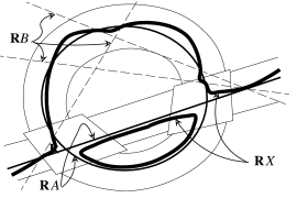
When depicting a topological plane curve one usually represents the projective plane either as a disc with opposite points of the boundary identified, or else as the compactification of $\mathbb{R}^{2}$, i.e., one visualizes the curve as its preimage under either the projection $D^{2}\to\mathbb{R}P^{2}$ or the inclusion $\mathbb{R}^{2}\to\mathbb{R}P^{2}$. In this book we shall use the second method. For example, 1 shows a curve corresponding to the symbol $\langle J\amalg 1\amalg 2\langle 1\rangle\amalg 1\langle 2\rangle\amalg 1 \langle 3\amalg 1\langle 2\rangle\rangle\rangle$.

1.3. Bézout’s Prohibitions and the Harnack Inequality
The most elementary prohibitions, it seems, are the topological consequences of Bézout’s theorem. In any case, these were the first prohibitions to be discovered.
1.3.A Bézout’s Theorem (see, for example, Wal-50, Sha-77).
Let $A_{1}$ and $A_{2}$ be nonsingular curves of degree $m_{1}$ and $m_{2}$. If the set $\mathbb{R}A_{1}\cap\,\mathbb{R}A_{2}$ is finite, then this set contains at most $m_{1}m_{2}$ points. If, in addition, $\mathbb{R}A_{1}$ and $\mathbb{R}A_{2}$ are transversal to one another, then the number of points in the intersection $\mathbb{R}A_{1}\cap\mathbb{R}A_{2}$ is congruent to $m_{1}m_{2}$ modulo 2.
1.3.B Corollary (1).
A nonsingular plane curve of degree $m$ is one-sided if and only if $m$ is odd. In particular, a curve of odd degree is nonempty.
In fact, in order for a nonsingular plane curve to be two-sided, i.e., to be homologous to zero $\mod 2$, it is necessary and sufficient that its intersection number with the projective line be zero $\mod 2$. By Bézout’s theorem, this is equivalent to the degree being even.$\square$
1.3.C Corollary (2).
The number of ovals in the union of two nests of a nonsingular plane curve of degree $m$ does not exceed $m/2$. In particular, a nest of a curve of degree $m$ has depth at most $m/2$, and if a curve of degree $m$ has a nest of depth $[m/2]$, then it does not have any ovals not in the nest.
To prove Corollary 2 it suffices to apply Bézout’s theorem to the curve and to a line which passes through the insides of the smallest ovals in the nests.$\square$
1.3.D Corollary (3).
There can be no more than $m$ ovals in a set of ovals which is contained in a union of $\leq 5$ nests of a nonsingular plane curve of degree $m$ and which does not contain an oval enveloping all of the other ovals of the set.
To prove Corollary 3 it suffices to apply Bézout’s theorem to the curve and to a conic which passes through the insides of the smallest ovals in the nests.$\square$
One can give corollaries whose proofs use curves of higher degree than lines and conics (see Section 3.8). The most important of such results is Harnack’s inequality.
1.3.E Corollary (4 (Harnack Inequality Har-76)).
The number of components of a nonsingular plane curve of degree $m$ is at most $\frac{(m-1)(m-2)}{2}+1$.
The derivation of Harnack Inequality from Bézout’s theorem can be found in Har-76, and also Gud-74. However, it is possible to prove Harnack Inequality without using Bézout’s theorem; see, for example, Gud-74, Wil-78 and Section 3.2 below.
1.4. Curves of Degree $\leq 5$
If $m\leq 5$, then it is easy to see that the prohibitions in the previous subsection are satisfied only by the following isotopy types.
$m$ Isotopy types of nonsingular plane curves of degree $m$ 1 $\langle J\rangle$ 2 $\langle 0\rangle,\,\langle 1\rangle$ 3 $\langle J\rangle,\,\langle J\amalg 1\rangle$ 4 $\langle 0\rangle,\,\langle 1\rangle,\,\langle 2\rangle,\,\langle 1\langle 1 \rangle\rangle,\,\langle 3\rangle,\,\langle 4\rangle$ 5 $\langle J\rangle,\,\langle J\amalg 1\rangle,\,\langle J\amalg 2\rangle,\, \langle J\amalg 1\langle 1\rangle\rangle,\,\langle J\amalg 3\rangle,\,\langle J \amalg 4\rangle,\,\langle J\amalg 5\rangle,\,\langle J\amalg 6\rangle$
For $m\leq 3$ the absence of other types follows from 1.3.B and 1.3.C; for $m=4$ it follows from 1.3.B, 1.3.C and 1.3.D, or else from 1.3.B, 1.3.C and 1.3.E; and for $m=5$ it follows from 1.3.B, 1.3.C and 1.3.E. It turns out that it is possible to realize all of the types in Table 1; hence, we have the following theorem.
1.4.A
Isotopy Classification of Nonsingular Real Plane Projective Curves of Degree $\leq 5$. An isotopy class of topological plane curves contains a nonsingular curve of degree $m\leq 5$ if and only if it occurs in the $m$-th row of Table 1.
The curves of degree $\leq 2$ are known to everyone. Both of the isotopy types of nonsingular curves of degree 3 can be realized by small perturbations of the union of a line and a conic which intersect in two real points (Figure 2). One can construct these perturbations by replacing the left side of the equation $cl=0$ defining the union of the conic $C$ and the line $L$ by the polynomial $cl+\varepsilon l_{1}l_{2}l_{3}$, where $l_{i}=0$, $i=1,2,3$, are the equations of the lines shown in 2, and $\varepsilon$ is a nonzero real number which is sufficiently small in absolute value.


It will be left to the reader to prove that one in fact obtains the curves in Figure 2 as a result; alternatively, the reader can deduce this fact from the theorem in the next subsection.
The isotopy types of nonempty nonsingular curves of degree 4 can be realized in a similar way by small perturbations of a union of two conics which intersect in four real points (Figure 3). An empty curve of degree 4 can be defined, for example, by the equation $x^{4}_{0}+x^{4}_{1}+x^{4}_{2}=0$.
All of the isotopy types of nonsingular curves of degree 5 can be realized by small perturbations of the union of two conics and a line, shown in Figure 4. $\square$
For the isotopy classification of nonsingular curves of degree 6 it is no longer sufficient to use this type of construction, or even the prohibitions in the previous subsection. See Section 1.13.
1.5. The Classical Method of Constructing Nonsingular Plane Curves
All of the classical constructions of the topology of nonsingular plane curves are based on a single construction, which I will call classical small perturbation. Some special cases were given in the previous subsection. Here I will give a detailed description of the conditions under which it can be applied and the results.
We say that a real singular point $\xi=(\xi_{0}:\xi_{1}:\xi_{2})$ of the curve $A$ is an intersection point of two real transversal branches, or, more briefly, a crossing,22Sometimes other names are used. For example: a node, a point of type $A_{1}$ with two real branches, a nonisolated nondegenerate double point. if the polynomial $a$ defining the curve has matrix of second partial derivatives at the point $(\xi_{0},\xi_{1},\xi_{2})$ with both a positive and a negative eigenvalue, or, equivalently, if the point $\xi$ is a nondegenerate critical point of index 1 of the functions $\{x\in\mathbb{R}P^{2}|x_{i}\neq 0\}\to\mathbb{R}\>x\mapsto a(x)/x_{i}\deg a$ for $i$ with $\xi_{i}\neq 0$. By Morse lemma (see, e.g. Mil-69) in a neighborhood of such a point the curve looks like a union of two real lines. Conversely, if $\mathbb{R}A_{1},\ldots,\mathbb{R}A_{k}$ are nonsingular mutually transverse curves no three of which pass through the same point, then all of the singular points of the union $\mathbb{R}A_{1}\cup\cdots\cup\mathbb{R}A_{k}$ (this is precisely the pairwise intersection points) are crossings.
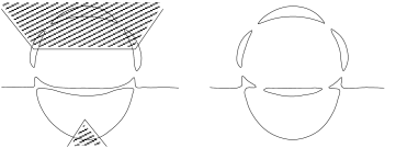
1.5.A Classical Small Perturbation Theorem (see Figure 5).
Let $A$ be a plane curve of degree $m$ all of whose singular points are crossings, and let $B$ be a plane curve of degree $m$ which does not pass through the singular points of $A$. Let $U$ be a regular neighborhood of the curve $\mathbb{R}A$ in $\mathbb{R}P^{2}$, represented as the union of a neighborhood $U_{0}$ of the set of singular points of $A$ and a tubular neighborhood $U_{1}$ of the submanifold $\mathbb{R}A\smallsetminus U_{0}$ in $\mathbb{R}P^{2}\smallsetminus U_{0}$.
Then there exists a nonsingular plane curve $X$ of degree $m$ such that:
(1) $\mathbb{R}X\subset U$.
(2) For each component $V$ of $U_{0}$ there exists a homeomorphism $h\>V\to D^{1}\times D^{1}$ such that $h(\mathbb{R}A\cap V)=D^{1}\times 0\cup 0\times D^{1}$ and $h(\mathbb{R}X\cap V)=\{(x,y)\in D^{1}\times D^{1}|xy=1/2\}$.
(3) $\mathbb{R}X\smallsetminus U_{0}$ is a section of the tubular fibration $U_{1}\to\mathbb{R}A\smallsetminus U_{0}$.
(4) $\mathbb{R}X\subset\{(x_{0}:x_{1}:x_{2})\in\mathbb{R}P^{2}|a(x_{0},x_{1},x_{2}) b(x_{0},x_{1},x_{2})\leq 0\}$, where $a$ and $b$ are polynomials defining the curves $A$ and $B$.
(5) $\mathbb{R}X\cap\mathbb{R}A=\mathbb{R}X\cap\mathbb{R}B=\mathbb{R}A\cap\mathbb{R}B$.
(6) If $p\in\mathbb{R}A\cap\mathbb{R}B$ is a nonsingular point of $B$ and $\mathbb{R}B$ is transversal to $\mathbb{R}A$ at this point, then $\mathbb{R}X$ is also transversal to $\mathbb{R}A$ at the point.
There exists $\varepsilon>0$ such that for any $t\in(0,\varepsilon]$ the curve given by the polynomial $a+tb$ satisfies all of the above requirements imposed on $X$.
It follows from (1)–(3) that for fixed $A$ the isotopy type of the curve $\mathbb{R}X$ depends on which of two possible ways it behaves in a neighborhood of each of the crossings of the curve $A$, and this is determined by condition (4). Thus, conditions (1)–(4) characterize the isotopy type of the curve $\mathbb{R}X$. Conditions (4)–(6) characterize its position relative to $\mathbb{R}A$.
We say that the curves defined by the polynomials $a+tb$ with $t\in(0,\varepsilon]$ are obtained by small perturbations of $A$ directed to the curve $B$. It should be noted that the curves $A$ and $B$ do not determine the isotopy type of the perturbed curves: since both of the polynomials $b$ and $-b$ determine the curve $B$, it follows that the polynomials $a-tb$ with small $t>0$ also give small perturbations of $A$ directed to $B$. But these curves are not isotopic to the curves given by $a+tb$ (at least not in $U)$, if the curve $A$ actually has singularities.
Proof.
Proof of Theorem 1.5.A We set $x_{t}=a+tb$. It is clear that for any $t\neq 0$ the curve $X_{t}$ given by the polynomial $x_{t}$ satisfies conditions (5) and (6), and if $t>0$ it satisfies (4). For small $|t|$ we obviously have $\mathbb{R}X_{t}\subset U$. Furthermore, if $|t|$ is small, the curve $\mathbb{R}X_{t}$ is nonsingular at the points of intersection $\mathbb{R}X_{t}\cap\mathbb{R}B=\mathbb{R}A\cap\mathbb{R}B$, since the gradient of $x_{t}$ differs very little from the gradient of $a$ when $|t|$ is small, and the latter gradient is nonzero on $\mathbb{R}A\cap\mathbb{R}B$ (this is because, by assumption, $B$ does not pass through the singular points of $A)$. Outside $\mathbb{R}B$ the curve $\mathbb{R}X_{t}$ is a level curve of the function $a/b$. On $\mathbb{R}A\smallsetminus\mathbb{R}B$ this level curve has critical points only at the singular points of $\mathbb{R}A$, and these critical points are nondegenerate. Hence, for small $t$ the behavior of $\mathbb{R}X_{t}$ outside $\mathbb{R}B$ is described by the implicit function theorem and Morse Lemma (see, for example, Mil-69); in particular, for small $t\neq 0$ this curve is nonsingular and satisfies conditions (2) and (3). Consequently, there exists $\varepsilon>0$ such that for any $t\in(0,\varepsilon]$ the curve $\mathbb{R}X_{t}$ is nonsingular and satisfies (1)–(6). $\square$
1.6. Harnack Curves
In 1876, Harnack Har-76 not only proved the inequality 1.3.E in Section 1.3, but also completed the topological classification of nonsingular plane curves by proving the following theorem.
1.6.A Harnack Theorem.
For any natural number $m$ and any integer $c$ satisfying the inequalities
| (1) | $\frac{1-(-1)^{m}}{2}\leq c\leq\frac{m^{2}-3m+4}{2},$ |
there exists a nonsingular plane curve of degree $m$ consisting of $c$ components.
The inequality on the right in 1 is Harnack Inequality. The inequality on the left is part of Corollary 1 of Bézout’s theorem (see Section 1.3.B). Thus, Harnack Theorem together with theorems 1.3.B and 1.3.E actually give a complete characterization of the set of topological types of nonsingular plane curves of degree $m$, i.e., they solve problem 1.1.A.
Curves with the maximum number of components (i.e., with $(m^{2}-3m+4)/2$ components, where $m$ is the degree) are called M-curves. Curves of degree $m$ which have $(m^{2}-3m+4)/2-a$ components are called $(M-a)$-curves. We begin the proof of Theorem 1.6.A by establishing that the Harnack Inequality 1.3.B is best possible.
1.6.B .
For any natural number $m$ there exists an M-curve of degree $m$.
Proof.
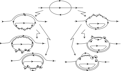
We shall actually construct a sequence of M-curves. At each step of the construction we add a line to the M-curve just constructed, and then give a slight perturbation to the union. We can begin the construction with a line or, as in Harnack’s proof in Har-76, with a circle. However, since we have already treated curves of degree $\leq 5$ and constructed M-curves for those degrees (see Section 1.4), we shall begin by taking the M-curve of degree 5 that was constructed in Section 1.4, so that we can immediately proceed to curves that we have not encountered before.
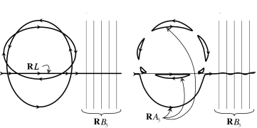
Recall that we obtained a degree 5 M-curve by perturbing the union of two conics and a line $L$. This perturbation can be done using various curves. For what follows it is essential that the auxiliary curve intersect $L$ in five points which are outside the two conics. For example, let the auxiliary curve be a union of five lines which satisfies this condition (Figure 6). We let $B_{5}$ denote this union, and we let $A_{5}$ denote the M-curve of degree 5 that is obtained using $B_{5}$.

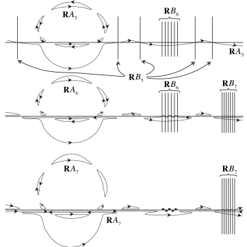
We now construct a sequence of auxiliary curves $B_{m}$ for $m>5$. We take $B_{m}$ to be a union of $m$ lines which intersect $L$ in $m$ distinct points lying, for even $m$, in an arbitrary component of the set $\mathbb{R}L\smallsetminus\mathbb{R}B_{m-1}$ and for odd $m$ in the component of $\mathbb{R}L\smallsetminus\mathbb{R}B_{m-1}$ containing $\mathbb{R}L\cap\mathbb{R}B_{m-2}$.

We construct the M-curve $A_{m}$ of degree $m$ using small perturbation of the union $A_{m-1}\cup L$ directed to $B_{m}$. Suppose that the M-curve $A_{m-1}$ of degree $m-1$ has already been constructed, and suppose that $\mathbb{R}A_{m-1}$ intersects $\mathbb{R}L$ transversally in the $m-1$ points of the intersection $\mathbb{R}L\cap\,\mathbb{R}B_{m-1}$ which lie in the same component of the curve $\mathbb{R}A_{m-1}$ and in the same order as on $\mathbb{R}L$. It is not hard to see that, for one of the two possible directions of a small perturbation of $A_{m-1}\cup L$ directed to $B_{m}$, the line $\mathbb{R}L$ and the component of $\mathbb{R}A_{m-1}$ that it intersects give $m-1$ components, while the other components of $\mathbb{R}A_{m-1}$, of which, by assumption, there are
| $((m-1)^{2}-3(m-1)+4)/2-1=(m^{2}-5m+6)/2,$ |
are only slightly deformed—so that the number of components of $\mathbb{R}A_{m}$ remains equal to $(m^{2}-5m+6)/2+m-1=(m^{2}-3m+4)/2$. We have thus obtained an M-curve of degree $m$. This curve is transversal to $\mathbb{R}L$, it intersects $\mathbb{R}L$ in $\mathbb{R}L\cap\mathbb{R}B_{m}$ (see 1.5.A), and, since $\mathbb{R}L\cap\mathbb{R}B_{m}$ is contained in one of the components of the set $\mathbb{R}L\smallsetminus\mathbb{R}B_{m-1}$, it follows that the intersection points of our curve with $\mathbb{R}L$ are all in the same component of the curve and are in the same order as on $\mathbb{R}L$ (Figure 7). $\square$
The proof that the left inequality in 1 is best possible, i.e., that there is a curve with the minimum number of components, is much simpler. For example, we can take the curve given by the equation $x^{m}_{0}+x^{m}_{1}+x^{m}_{2}=0$. Its set of real points is obviously empty when $m$ is even, and when $m$ is odd the set of real points is homeomorphic to $\mathbb{R}P^{1}$ (we can get such a homeomorphism onto $\mathbb{R}P^{1}$, for example, by projection from the point $(0:0:1))$.
By choosing the auxiliary curves $B_{m}$ in different ways in the construction of M-curves in the proof of Theorem 1.6.B, we can obtain curves with any intermediate number of components. However, to complete the proof of Theorem 1.6.A in this way would be rather tedious, even though it would not require any new ideas. We shall instead turn to a less explicit, but simpler and more conceptual method of proof, which is based on objects and phenomena not encountered above.
1.7. Digression: the Space of Real Projective Plane Curves
By the definition of real projective algebraic plane curves of degree $m$, they form a real projective space of dimension $m(m+3)/2$. The homogeneous coordinates in this projective space are the coefficients of the polynomials defining the curves. We shall denote this space by the symbol $\mathbb{R}C_{m}$. Its only difference with the standard space $\mathbb{R}P^{m(m+3)/2}$ is the unusual numbering of the homogeneous coordinates. The point is that the coefficients of a homogeneous polynomial in three variables have a natural double indexing by the exponents of the monomials:
| $a(x_{0},x_{1},x_{2})=\sum\substack{i,j\geq 0\\ i+j\leq m}a_{ij}x^{m-i-j}_{0}x^{i}_{1}x^{j}_{2}.$ |
We let $\mathbb{R}NC_{m}$ denote the subset of $\mathbb{R}C_{m}$ corresponding to the real nonsingular curves. It is obviously open in $\mathbb{R}C_{m}$. Moreover, any nonsingular curve of degree $m$ has a neighborhood in $\mathbb{R}NC_{m}$ consisting of isotopic nonsingular curves. Namely, small changes in the coefficients of the polynomial defining the curve lead to polynomials which give smooth sections of a tubular fibration of the original curve. This is an easy consequence of the implicit function theorem; compare with 1.5.A, condition (3).
Curves which belong to the same component of the space $\mathbb{R}NC_{m}$ of nonsingular degree $m$ curves are isotopic—this follows from the fact that nonsingular curves which are close to one another are isotopic. A path in $\mathbb{R}NC_{m}$ defines an isotopy in $\mathbb{R}P^{2}$ of the set of real points of a curve. An isotopy obained in this way is made of sets of real points of of real points of curves of degree $m$. Such an isotopy is said to be rigid. This definition naturally gives rise to the following classification problem, which is every bit as classical as problems 1.1.Aand 1.1.B.
1.7.A Rigid Isotopy Classification Problem.
Classify the nonsingularcurves of degree $m$ up to rigid isotopy, i.e., study the partition of the space $\mathbb{R}NC_{m}$ of nonsingular degree $m$ curves into its components.
If $m\leq 2$, it is well known that the solution of this problem is identical to that of problem 1.1.B. Isotopy also implies rigid isotopy for curves of degree 3 and 4. This was known in the last century; however, we shall not discuss this further here, since it has little relevance to what follows. At present problem 1.7.A has been solved for $m\leq 6$.
Although this section is devoted to the early stages of the theory, I cannot resist commenting in some detail about a more recent result. In 1978, V. A. Rokhlin Rok-78 discovered that for $m\geq 5$ isotopy of nonsingular curves of degree $m$ no longer implies rigid isotopy. The simplest example is given in Figure 8, which shows two curves of degree 5. They are obtained by slightly perturbing the very same curve in Figure 4 which is made up of two conics and a line. Rokhlin’s original proof uses argument on complexification, it will be presented below, in Section ??? Here, to prove that these curves are not rigid isotopic, we use more elementary arguements. Note that the first curve has an oval lying inside a triangle which does not intersect the one-sided component and which has its vertices inside the other three ovals, and the second curve does not have such an oval—but under a rigid isotopy the oval cannot leave the triangle, since that would entail a violation of Bézout’s theorem.
We now examine the subset of $\mathbb{R}C_{m}$ made up of real singular curves.
It is clear that a curve of degree $m$ has a singularity at $(1:0:0)$ if and only if its polynomial has zero coefficients of the monomials $x^{m}_{0},x^{m-1}_{0}x_{1},x^{m-1}_{0}x_{2}$. Thus, the set of real projective plane curves of degree $m$ having a singularity at a particular point forms a subspace of codimension 3 in $\mathbb{R}C_{m}$.
We now consider the space $S$ of pairs of the form $(p,C)$, where $p\in\mathbb{R}P^{2}$, $C\in\mathbb{R}C_{m}$, and $p$ is a singular point of the curve $C$. $S$ is clearly an algebraic subvariety of the product $\mathbb{R}P^{2}\times\mathbb{R}C_{m}$. The restriction to $S$ of the projection $\mathbb{R}P^{2}\times\mathbb{R}C_{m}\to\mathbb{R}P^{2}$ is a locally trivial fibration whose fiber is the space of curves of degree $m$ with a singularity at the corresponding point, i.e., the fiber is a projective space of dimension $m(m+3)/2-3$. Thus, $S$ is a smooth manifold of dimension $m(m+3)/2-1$. The restriction $S\to\mathbb{R}C_{m}$ of the projection $\mathbb{R}P^{2}\times\mathbb{R}C_{m}\to\mathbb{R}C_{m}$ has as its image precisely the set of all real singular curves of degree $m$, i.e., $\mathbb{R}C_{m}\smallsetminus\mathbb{R}NC_{m}$. We let $\mathbb{R}SC_{m}$ denote this image. Since it is the image of a $(m(m+3)/2-1)$-dimensional manifold under smooth map, its dimension is at most $m(m+3)/2-1$. On the other hand, its dimension is at least equal $m(m+3)/2-1$, since otherwise, as a subspace of codimension $\geq 2$, it would not separate the space $\mathbb{R}C_{m}$, and all nonsingular curves of degree $m$ would be isotopic.
Using an argument similar to the proof that $\dim\mathbb{R}SC_{m}\leq m(m+3)/2-1$, one can show that the set of curves having at least two singular points and the set of curves having a singular point where the matrix of second derivatives of the corresponding polynomial has rank $\leq 1$, each has dimension at most $m(m+3)/2-2$. Thus, the set $\mathbb{R}SC_{m}$ has an open everywhere dense subset consisting of curves with only one singular point, which is a nondegenerate double point (meaning that at this point the matrix of second derivatives of the polynomial defining the curve has rank 2). This subset is called the principal part of the set $\mathbb{R}SC_{m}$. It is a smooth submanifold of codimension 1 in $\mathbb{R}C_{m}$. In fact, its preimage under the natural map $S\to\mathbb{R}C_{m}$ is obviously an open everywhere dense subset in the manifold $S$, and the restriction of this map to the preimage is easily verified to be a one-to-one immersion, and even a smooth imbedding.
There are two types of nondegenerate real points on a plane curve. We say that a nondegenerate real double point $(\xi_{0}:\xi_{1}:\xi_{2})$ on a curve $A$ is solitary if the matrix of second partial derivatives of the polynomial defining $A$ has either two nonnegative or two nonpositive eigenvalues at the point $(\xi_{0},\xi_{1},\xi_{2})$. A solitary nondegenerate double point of $A$ is an isolated point of the set $\mathbb{R}A$. In general, a singular point of $A$ which is an isolated point of the set $\mathbb{R}A$ will be called a solitary real singular point. The other type of nondegenerate real double point is a crossing; crossings were discussed in Section 1.5 above. Corresponding to this division of the nondegenerate real double points into solitary points and crossings, we have a partition of the principal part of the set of real singular curves of degree $m$ into two open sets.
If a curve of degree $m$ moves as a point of $\mathbb{R}C_{m}$ along an arc which has a transversal intersection with the half of the principal part of the set of real singular curves consisting of curves with a solitary singular point, then the set of real points on this curve undergoes a Morse modification of index 0 or 2 (i.e., either the curve acquires a solitary double point, which then becomes a new oval, or else one of the ovals contracts to a point (a solitary nondegenerate double point) and disappears). In the case of a transversal intersection with the other half of the principal part of the set of real singular curves one has a Morse modification of index 1 (i.e., two arcs of the curve approach one another and merge, with a crossing at the point where they come together, and then immediately diverge in their modified form, as happens, for example, with the hyperbola in the family of affine curves of degree 2 given by the equation $xy=t$ at the moment when $t=0)$.
A line in $\mathbb{R}C_{m}$ is called a (real) pencil of curves of degree $m$. If $a$ and $b$ are polynomials defining two curves of the pencil, then the other curves of the pencil are given by polynomials of the form $\lambda a+\mu b$ with $\lambda,\mu\in\mathbb{R}\smallsetminus 0$.
By the transversality theorem, the pencils which intersect the set of real singular curves only at points of the principal part and only transversally form an open everywhere dense subset of the set of all real pencils of curves of degree $m$.
1.8. End of the Proof of Theorem 1.6.A
In Section 1.6 it was shown that for any $m$ there exist nonsingular curves of degree $m$ with the minimum number $(1-(-1)^{m})/2$ or with the maximum number $(m^{2}-3m+4)/2$ of components. Nonsingular curves which are isotopic to one another form an open set in the space $\mathbb{R}C_{m}$ of real projective plane curves of degree $m$ (see Section 1.7). Hence, there exists a real pencil of curves of degree $m$ which connects a curve with minimum number of components to a curve with maximum number of components and which intersects the set of real singular curves only in its principal part and only transversally. As we move along this pencil from the curve with minimum number of components to the curve with maximum number of components, the curve only undergoes Morse modifications, each of which changes the number of components by at most 1. Consequently, this pencil includes nonsingular curves with an arbitrary intermediate number of components.$\square$
1.9. Isotopy Types of Harnack M-Curves
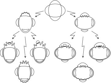
Harnack’s construction of M-curves in Har-76 differs from the construction in the proof of Theorem 1.6.B in that a conic, rather than a curve of degree 5, is used as the original curve. Figure 9 shows that the M-curves of degree $\leq 5$ which are used in Harnack’s construction Har-76. For $m\geq 6$ Harnack’s construction gives M-curves with the same isotopy types as in the construction in Section 1.6.

In these constructions one obtains different isotopy types of M-curves depending on the choice of auxiliary curves (more precisely, depending on the relative location of the intersections $\mathbb{R}B_{m}\cap\mathbb{R}L)$. Recall that in order to obtain M-curves it is necessary for the intersection $\mathbb{R}B_{m}\cap\mathbb{R}L$ to consist of $m$ points and lie in a single component of the set $\mathbb{R}L\smallsetminus\mathbb{R}B_{m-1}$, where for odd $m$ this component must contain $\mathbb{R}B_{m-2}\cap\mathbb{R}L$. It is easy to see that the isotopy type of the resulting M-curve of degree $m$ depends only on the choice of the components of $\mathbb{R}L\smallsetminus\mathbb{R}B_{r-1}$ for even $r<m$ where the intersections $\mathbb{R}L\cap\mathbb{R}B_{r}$ are to be found. If we take the components containing $\mathbb{R}L\cap\mathbb{R}B_{r-2}$ for even $r$ as well, then the degree $m$ M-curve obtained from the construction has isotopy type $\langle J\amalg(m^{2}-3m+2)/2\rangle$ for odd $m$ and $\langle(3m^{2}-6m)/8\amalg 1\langle(m^{2}-6m+8)/8\rangle\rangle$ for even $m$. In Table 2 we have listed the isotopy types of M-curves of degree $\leq 10$ which one obtains from Harnack’s construction using all possible $B_{m}$.
$m$ Isotopy types of the Harnack M-curves of degree $m$ 2 $\langle 1\rangle$ 3 $\langle J\amalg 1\rangle$ 4 $\langle 4\rangle$ 5 $\langle J\amalg 6\rangle$ 6 $\langle 9\amalg 1\langle 1\rangle\rangle$ 7 $\langle J\amalg 15\rangle\qquad\langle J\amalg 13\amalg 1\langle 1\rangle\rangle$ 8 $\langle 18\amalg 1\langle 3\rangle\rangle\qquad\qquad\qquad\langle 17\amalg 1 \langle 1\rangle\amalg 1\langle 2\rangle\rangle$ 9 $\langle J\amalg 28\rangle\qquad\langle J\amalg 24\amalg 1\langle 3\rangle \rangle\qquad\quad\langle J\amalg 26\amalg 1\langle 1\rangle\rangle\qquad \langle J\amalg 23\amalg 1\langle 1\rangle\amalg 1\langle 2\rangle\rangle$ 10 $\langle 30\amalg 1\langle 6\rangle\rangle\qquad\langle 29\amalg 2\langle 3 \rangle\rangle\qquad\quad\langle 29\amalg 1\langle 1\rangle\amalg 1\langle 5 \rangle\rangle\qquad\langle 28\amalg 1\langle 1\rangle\amalg 1\langle 2\rangle \amalg 1\langle 3\rangle\rangle$
In conclusion, we mention two curious properties of Harnack M-curves, for which the reader can easily furnish a proof.
1.9.A .
The depth of a nest in a Harnack M-curve is at most 2.
1.9.B .
Any Harnack M-curve of even degree $m$ has $(3m^{2}-6m+8)/8$ outer ovals and $(m^{2}-6m+8)/8$ inner ovals.
1.10. Hilbert Curves
In 1891 Hilbert Hil-91 seems to have been the first to clearly state the isotopy classification problem for nonsingular curves. As we saw, the isotopy types of Harnack M-curves are very special. Hilbert suggested that from the topological viewpoints M-curves are the most interesting. This Hilbert’s guess was strongly confirmed by the whole subsequent development of the field.
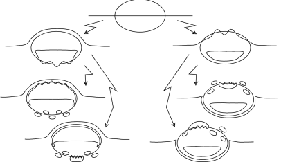
There is a big gap between property 1.9.A of Harnack M-curves and the corresponding prohibition in 1.3.C. Hilbert Hil-91 showed that this gap is explained by the peculiarities of the construction and not by the intrinsic properties of M-curves. He proposed a new method of constructing M-curves which was close to Harnack’s method, but which gives M-curves with nests of any depth allowed by Theorem 1.3.C. In his method the role a line plays in Harnack’s method is played instead by a nonsingular conic, and a line or a conic is used for the starting curve. Figures 10–11 show how to construct M-curves by Hilbert’s method.
In Table 3 we list the isotopy types of M-curves of degree $\leq 8$ which are obtained by Hilbert’s construction.
$m$ Isotopy types of the Hilbert M-curves of degree $m$ 4 $\langle 1\rangle$ 6 $\langle 9\amalg 1\langle 1\rangle\rangle\qquad\qquad\qquad\langle 1\amalg 1 \langle 9\rangle\rangle$ 8 $\langle 5\amalg 1\langle 14\amalg 1\langle 1\rangle\rangle\rangle\ \langle 17 \amalg 1\langle 2\amalg 1\langle 1\rangle\rangle\rangle\ \langle 18\amalg 1 \langle 3\rangle\rangle$ $\langle 1\amalg 1\langle 2\amalg 1\langle 17\rangle\rangle\rangle\ \langle 1 \amalg 1\langle 14\amalg 1\langle 5\rangle\rangle\rangle$ 5 $\langle J\amalg 6\rangle$ 7 $\langle J\amalg 15\rangle\quad\langle J\amalg 12\amalg 1\langle 2\rangle \rangle\quad\langle J\amalg 13\amalg 1\langle 3\rangle\rangle\quad\langle J \amalg 2\amalg 1\langle 12\rangle\rangle\quad\langle J\amalg 1\amalg 1\langle 1 3\rangle\rangle$
The first difficult special problems that Hilbert met were related with curves of degree 6. Hilbert succeeded to construct M-curves of degree $\geq 6$ with mutual position of components different from the scheme $\langle 9\amalg 1\langle 1\rangle\rangle$ realized by Harnack. However he realized only one new real scheme of degree 6, namely $\langle 1\amalg 1\langle 9\rangle\rangle$. Hilbert conjectured that these are the only real schemes realizable by M-curves of degree 6 and for a long time affirmed that he had a (long) proof of this conjecture. Even being false (it was disproved by D. A. Gudkov in 1969, who constructed a curve with the scheme $\langle 5\amalg 1\langle 5\rangle\rangle$) this conjecture caught the things that became in 30-th and 70-th the core of the theory.
In fact, Hilbert invented a method which allows to answer to all questions on topology of curves of degree 6. It involves a detailed analysis of singular curves which could be obtained from a given nonsingular one. The method required complicated fragments of singularity theory, which had not been elaborated at the time of Hilbert. Completely this project was realized only in the sixties by D. A. Gudkov. It was Gudkov who obtained a complete table of real schemes of curves of degree 6.
Coming back to Hilbert, we have to mention his famous problem list Hil-01. He included into the list, as a part of the sixteenth problem, a general question on topology of real algebraic varieties and more special questions like the problem on mutual position of components of a plane curve of degree 6.
The most mysterious in this problem seems to be its number. The number sixteen plays a very special role in topology of real algebraic varieties. It is difficult to believe that Hilbert was aware of that. It became clear only in the beginning of seventies (see Rokhlin’s paper “Congruences modulo sixteen in the sixteenth Hilbert’s problem” Rok-72). Nonetheless, sixteen was the number assigned by Hilbert to the problem.
1.11. Analysis of the Results of the Constructions. Ragsdale
In 1906, V. Ragsdale Rag-06 made a remarkable attempt to guess new prohibitions, based on the results of the constructions by Harnack’s and Hilbert’s methods. She concentrated her attention on the case of curves of even degree, motivated by the following special properties of such curves. Since a curve of an even degree is two-sided, it divides $\mathbb{R}P^{2}$ into two parts, which have the curve as their common boundary. One of the parts contains a nonorientable component; it is denoted by $\mathbb{R}P^{2}_{-}$. The other part, which is orientable, is denoted by $\mathbb{R}P^{2}_{+}$. The ovals of a curve of even degree are divided into inner and outer ovals with respect to $\mathbb{R}P^{2}_{+}$ (i.e., into ovals which bound a component of $\mathbb{R}P^{2}_{+}$ from the inside and from the outside). Following Petrovsky Pet-38, one says that the outer ovals with respect to $\mathbb{R}P^{2}_{+}$ are the even ovals (since such an oval lies inside an even number of other ovals), and the rest of the ovals are called odd ovals. The number of even ovals is denoted by $p$, and the number of odd ovals is denoted by $n$. These numbers contain very important information about the topology of the sets $\mathbb{R}P^{2}_{+}$ and $\mathbb{R}P^{2}_{-}$. Namely, the set $\mathbb{R}P^{2}_{+}$ has $p$ components, the set $\mathbb{R}P^{2}_{-}$ has $n+1$ components, and the Euler characteristics are given by $\chi(\mathbb{R}P^{2}_{+})=p-n$ and $\chi(\mathbb{R}P^{2}_{-})=n-p+1$. Hence, one should pay special attention to the numbers $p$ and $n$. (It is amazing that essentially these considerations were stated in a paper in 1906!)
By analyzing the constructions, Ragsdale Rag-06 made the following observations.
1.11.A (compare with 1.9.A and 1.9.B).
For any Harnack M-curve of even degree $m$,
| $p=(3m^{2}-6m+8)/8,\qquad n=(m^{2}-6m+8)/8.$ |
1.11.B .
For any Hilbert M-curve of even degree $m$,
| $\displaystyle(m^{2}-6m+16)/8\leq p\leq(3m^{2}-6m+8)/8,$ | ||
| $\displaystyle(m^{2}-6m+8)/8\leq n\leq(3m^{2}-6m)/8.$ |
This gave her evidence for the following conjecture.
1.11.C Ragsdale Conjecture.
For any curve of even degree $m$,
| $p\leq(3m^{2}-6m+8)/8,\qquad n\leq(3m^{2}-6m)/8.$ |
The most mysterious in this problem seems to be its number. The number sixteen plays a very special role in topology of real algebraic varieties. It is difficult to believe that Hilbert was aware of that. It became clear only in the beginning of seventies (see Rokhlin’s paper “Congruences modulo sixteen in the sixteenth Hilbert’s problem” Rok-72). Nonetheless, sixteen was the number assigned by Hilbert to the problem.
Writing cautiously, Ragsdale formulated also weaker conjectures. About thirty years later I. G. Petrovsky Pet-33, Pet-38 proved one of these weaker conjectures. See below Subsection 1.13.
Petrovsky also formulated conjectures about the upper bounds for $p$ and $n$. His conjecture about $n$ was more cautious (by 1).
Both Ragsdale Conjecture formulated above and its version stated by Petrovsky Pet-38 are wrong. However they stayed for rather long time: Ragsdale Conjecture on $n$ was disproved by the author of this book Vir-80 in 1979. However the disproof looked rather like improvement of the conjecture, since in the counterexamples $n=\frac{3k(k-1)}{2}+1$. Drastically Ragsdale-Petrovsky bounds were disproved by I. V. Itenberg Ite-93 in 1993: in Itenberg’s counterexamples the difference between $p$ (or $n$) and $\frac{3k(k-1)}{2}+1$ is a quadratic function of $k$.
In Section LABEL:s5.4s we shall return to this very first conjecture of a general nature on the topology of real algebraic curves. At this point we shall only mention that several weaker assertions have been proved and examples have been constructed which made it necessary to weaken the second inequality by 1. In the weaker form the Ragsdale conjecture has not yet been either proved or disproved.
The numbers $p$ and $n$ introduced by Ragsdale occur in many of of the prohibitions that were subsequently discovered. While giving full credit to Ragsdale for her insight, we must also say that, if she had looked more carefully at the experimental data available to her, she should have been able to find some of these prohibitions. For example, it is not clear what stopped her from making the conjecture which was made by Gudkov GU-69 in the late 1960’s. In particular, the experimental data could suggest the formulation of the Gudkov-Rokhlin congruence proved in Rok-72: for any M-curve of even degree $m=2k$
| $p-n\equiv k^{2}\mod 8$ |
Maybe mathematicians trying to conjecture restrictions on some integer should keep this case in mind as an evidence that restrictions can have not only the shape of inequality, but congruence. Proof of these Gudkov’s conjectures initiated by Arnold Arn-71 and completed by Rokhlin Rok-72, Kharlamov Kha-73, Gudkov and Krakhnov GK-73 had marked the beginning of the most recent stage in the development of the topology of real algebraic curves. We shall come to this story at the end of this Section.
1.12. Generalizations of Harnack’s and Hilbert’s Methods. Brusotti. Wiman
Ragsdale’s work Rag-06 was partly inspired by the erroneous paper of Hulbrut, containing a proof of the false assertion that an M-curve can be obtained by means of a classical small perturbation (see Section 1.5) from only two M-curves, one of which must have degree $\leq 2$. If this had been true, it would have meant that an inductive construction of M-curves by classical small perturbations starting with curves of small degree must essentially be either Harnack’s method or Hilbert’s method.
In 1910–1917, L. Brusotti showed that this is not the case. He found inductive constructions of M-curves based on classical small perturbation which were different from the methods of Harnack and Hilbert.
Before describing Brusotti’s constructions, we need some definitions. A simple arc $X$ in the set of real points of a curve $A$ of degree $m$ is said to be a base of rank $\rho$ if there exists a curve of degree $\rho$ which intersects the arc in $\rho m$ (distinct) points. A base of rank $\rho$ is clearly also a base of rank any multiple of $\rho$ (for example, one can obtain the intersecting curve of the corresponding degree as the union of several copies of the degree $\rho$ curve, each copy shifted slightly).
An M-curve $A$ is called a generating curve if it has disjoint bases $X$ and $Y$ whose ranks divide twice the degree of the curve. An M-curve $A_{0}$ of degree $m_{0}$ is called an auxiliary curve for the generating curve $A$ of degree $m$ with bases $X$ and $Y$ if the following conditions hold:
a) The intersection $\mathbb{R}A\cap\mathbb{R}A_{0}$ consist of $mm_{0}$ distinct points and lies in a single component $K$ of $\mathbb{R}A$ and in a single component $K$ of $\mathbb{R}A_{0}$.
b) The cyclic orders determined on the intersection $\mathbb{R}A\cap\mathbb{R}A_{0}$ by how it is situated in $K$ and in $K_{0}$ are the same.
c) $X\subset\mathbb{R}A\smallsetminus\mathbb{R}A_{0}$.
d) If $K$ is a one-sided curve and $m_{0}\equiv\mod 2$, then the base $X$ lies outside the oval $K_{0}$.
e) The rank of the base $X$ is a divisor of the numbers $m+m_{0}$ and $2m$, and the rank of $Y$ is a divisor of $2m+m_{0}$ and $2m$.
An auxiliary curve can be the empty curve of degree 0. In this case the rank of $X$ must be a divisor of the degree of the generating curve.
Let $A$ be a generating curve of degree $m$, and let $A_{0}$ be a curve of degree $m_{0}$ which is an auxiliary curve with respect to $A$ and the bases $X$ and $Y$. Since the rank of $X$ divides $m+m_{0}$, we may assume that the rank is equal to $m+m_{0}$. Let $C$ be a real curve of degree $m+m_{0}$ which intersects $X$ in $m(m+m_{0})$ distinct points. It is not hard to verify that a classical small perturbation of the curve $A\cup A_{0}$ directed to $L$ will give an M-curve of degree $m+m_{0}$, and that this M-curve will be an auxiliary curve with respect to $A$ and the bases obtained from $Y$ and $X$ (the bases must change places). We can now repeat this construction, with $A_{0}$ replaced by the curve that has just been constructed. Proceeding in this way, we obtain a sequence of M-curves whose degree forms an arithmetic progression: $km+m_{0}$ with $k=1,2,\ldots$. This is called the construction by Brusotti’s method, and the sequence of M-curves is called a Brusotti series.
Any simple arc of a curve of degree $\leq 2$ is a base of rank 1 (and hence of any rank). This is no longer the case for curves of degree $\leq 3$. For example, an arc of a curve of degree 3 is a base of rank 1 if and only if it contains a point of inflection. (We note that a base of rank 2 on a curve of degree 3 might not contain a point of inflection: it might be on the oval rather than on the one-sided component where all of the points of inflection obviously lie. A curve of degree 3 with this type of base of rank 2 can be constructed by a classical small perturbation of a union of three lines.)
If the generating curve has degree 1 and the auxiliary curve has degree 2, then the Brusotti construction turns out to be Harnack’s construction. The same happens if we take an auxiliary curve of degree 1 or 0. If the generating curve has degree 2 and the auxiliary curve has degree 1 or 2 (or 0), then the Brusotti construction is the same as Hilbert’s construction.
In general, not all Harnack and Hilbert constructions are included in Brusotti’s scheme; however, the Brusotti construction can easily be extended in such a way as to be a true generalization of the Harnack and Hilbert constructions. This extension involves allowing the use of an arbitrary number of bases of the generating curve. Such an extension is particularly worthwhile when the generating curve has degree $\leq 2$, in which case there are arbitrarily many bases.
It can be shown that Brusotti’s construction with generating curve of degree 1 and auxiliary curve of degree $\leq 4$ gives the same types of M-curves as Harnack’s construction. But as soon as one uses auxiliary curves of degree 5, one can obtain new isotopy types from Brusotti’s construction. It was only in 1971 that Gudkov Gud-71 found an auxiliary curve of degree 5 that did this. His construction was rather complicated, and so I shall only give some references Gud-71, Gud-74, A’C-79 and present Figure 12, which illustrates the location of the degree 5 curve relative to the generating line.


Even with the first stage of Brusotti’s construction, i.e., the classical small perturbation of the union of the curve and the line, one obtains an M-curve (of degree 6) which has isotopy type $\langle 5\amalg 1\langle 5\rangle\rangle$, an isotopy type not obtained using the constructions of Harnack and Hilbert. Such an M-curve of degree 6 was first constructed in a much more complicated way by Gudkov GU-69, Gud-73 in the late 1960’s.
In Figures 13 and 14 we show the construction of two curves of degree 6 which are auxiliary curves with respect to a line. In this case the Brusotti construction gives new isotopy types beginning with degree 8.

In the Hilbert construction we keep track of the location relative to a fixed line $A$. The union of two conics is perturbed in direction to a quadruple of lines. One obtains a curve of degree 4. To this curve one then adds one of the original conics, and the union is perturbed.
In numerous papers by Brusotti and his students, many series of Brusotti M-curves were found. Generally, new isotopy types appear in them beginning with degree 9 or 10. In these constructions they paid much attention to combinations of nests of different depths—a theme which no longer seems to be very interesting. An idea of the nature of the results in these papers can be obtained from Gudkov’s survey Gud-74; for more details, see Brusotti’s survey Bru-56 and the papers cited there.
An important variant of the classical constructions of M-curves, of which we shall need to make use in the next section, is not subsumed under Brusotti’s scheme even in its extended form. This variant, proposed by Wiman Wim-23, consists in the following. We take an M-curve $A$ of degree $k$ having base $X$ of rank dividing $k$; near this curve we construct a curve $A^{\prime}$ transversally intersecting $A$ in $k^{2}$ points of $X$, after which we can subject the union $A\cup A^{\prime}$ to a classical small perturbation, giving an M-curve of degree $2k$ (for example, a perturbation in direction to an empty curve of degree $2k)$. The resulting M-curve has the following topological structure: each of the components of the curve $A$ except for one (i.e., except for the component containing $X)$ is doubled, i.e., is replaced by a pair of ovals which are each close to an oval of the original curve, and the component containing $X$ gives a chain of $k^{2}$ ovals. This new curve does not necessarily have a base, so that in general one cannot construct a series of M-curves in this way.
1.13. The First Prohibitions not Obtained from Bézout’s Theorem
The techniques discussed above are, in essence, completely elementary. As we saw (Section 1.4), they are sufficient to solve the isotopy classification problem for nonsingular projective curves of degree $\leq 5$. However, even in the case of curves of degree 6 one needs subtler considerations. Not all of the failed attempts to construct new isotopy types of M-curves of degree 6 (after Hilbert’s 1891 paper Hil-91, there were two that had not been realized: $\langle 9\amalg 1\langle 1\rangle\rangle$ and $\langle 1\amalg 1\langle 9\rangle\rangle)$ could be explained on the basis of Bézout’s theorem. Hilbert undertook an attack on M-curves of degree 6. He was able to grope his way toward a proof that isotopy types cannot be realized by curves of degree 6, but the proof required a very involved investigation of the natural stratification of the space $\mathbb{R}C_{6}$ of real curves of degree 6. In Roh-13, Rohn, developing Hilbert’s approach, proved (while stating without proof several valid technical claims which he needed) that the types $\langle 11\rangle$ and $\langle 1\langle 10\rangle\rangle$ cannot be realized by curves of degree 6. It was not until the 1960’s that the potential of this approach was fully developed by Gudkov. By going directly from Rohn’s 1913 paper Roh-13 to the work of Gudkov, I would violate the chronological order of my presentation of the history of prohibitions. But in fact I would only be omitting one important episode, to be sure a very remarkable one: the famous work of I. G. Petrovsky Pet-33, Pet-38 in which he proved the first prohibition relating to curves of arbitrary even degree and not a direct consequence of Bézout’s theorem.
1.13.A Petrovsky Theorem (Pet-33, Pet-38).
For any nonsingular real projective algebraic plane curve of degree $m=2k$
| (2) | $-\frac{3}{2}k(k-1)\leq p-n\leq\frac{3}{2}k(k-1)+1.$ |
(Recall that $p$ denotes the number of even ovals on the curve (i.e., ovals each of which is enveloped by an even number of other ovals, see Section 1.11), and $n$ denotes the number of odd ovals.)
As it follows from Pet-33 and Pet-38, Petrovsky did not know Ragsdale’s paper. But his proof runs along the lines indicated by Ragsdale. He also reduced the problem to estimates of Euler characteristic of the pencil curves, but he went further: he proved these estimates. Petrovsky’s proof was based on a technique that was new in the study of the topology of real curves: the Euler-Jacobi interpolation formula. Petrovsky’s theorem was generalized by Petrovsky and Oleinik PO-49 to the case of varieties of arbitrary dimension, and by Oleĭnik Ole-51 to the case of curves on a surface. More about the proof and the influence of Petrovsky’s work on the subsequent development of the subject can be found in Kharlamov’s survey Kha-86 in Petrovsky’s collected works. I will only comment that in application to nonsingular projective plane curves, the full potential of Petrovsky’s method, insofar as we are able to judge, was immediately realized by Petrovsky himself.
We now turn to Gudkov’s work. In a series of papers in the 1950’s and 1960’s, he completed the development of the techniques needed to realize Hilbert’s approach to the problem of classifying curves of degree 6 (these techniques were referred to as the Hilbert-Rohn method by Gudkov), and he used the techniques to solve this problem (see GU-69). The answer turned out to be elegant and stimulating.
1.13.B Gudkov’s Theorem GU-69.
The 56 isotopy types listed in Table 4, and no others, can be realized by nonsingular real projective algebraic plane curves of degree 6.
| $\displaystyle\ \ \langle 9\amalg 1\langle 1\rangle\rangle\phantom{ \langle 9\amalg 1\langle 1\rangle\rangle\ \langle 9\amalg 1\langle 1 \rangle\rangle\ \langle 9\amalg 1\langle 1\rangle\rangle}\ \langle 5 \amalg 1\langle 5\rangle\rangle\ \phantom{\langle 9\amalg 1\langle 1 \rangle\rangle\ \langle 9\amalg 1\langle 1\rangle\rangle\ \langle 9 \amalg 1\langle 1\rangle\rangle}\ \langle 1\amalg 1\langle 9\rangle\rangle$ | ||
| $\displaystyle\langle 10\rangle\ \langle 8\amalg 1\langle 1\rangle\rangle \ \phantom{\langle 9\amalg 1\langle 1\rangle\rangle\ \langle 9\amalg 1 \langle 1\rangle\rangle}\ \langle 5\amalg 1\langle 4\rangle\rangle\ \langle 4\amalg 1\langle 5\rangle\rangle\ \phantom{\langle 9\amalg 1 \langle 1\rangle\rangle\ \langle 9\amalg 1\langle 1\rangle\rangle}\ \langle 1\amalg 1\langle 8\rangle\rangle\ \langle 1\langle 9\rangle\rangle$ | ||
| $\displaystyle\langle 9\rangle\ \langle 7\amalg 1\langle 1\rangle\rangle \ \langle 6\amalg 1\langle 2\rangle\rangle\ \langle 5\amalg 1\langle 3 \rangle\rangle\ \langle 4\amalg 1\langle 4\rangle\rangle\ \langle 3 \amalg 1\langle 5\rangle\rangle\ \langle 2\amalg 1\langle 6\rangle\rangle \ \langle 1\amalg 1\langle 7\rangle\rangle\ \langle 1\langle 8\rangle\rangle$ | ||
| $\displaystyle\langle 8\rangle\ \langle 6\amalg 1\langle 1\rangle\rangle \ \langle 5\amalg 1\langle 2\rangle\rangle\ \langle 4\amalg 1\langle 3 \rangle\rangle\ \langle 3\amalg 1\langle 4\rangle\rangle\ \langle 2 \amalg 1\langle 5\rangle\rangle\ \langle 1\amalg 1\langle 6\rangle\rangle \ \langle 1\langle 7\rangle\rangle$ | ||
| $\displaystyle\langle 7\rangle\ \langle 5\amalg 1\langle 1\rangle\rangle \ \langle 4\amalg 1\langle 2\rangle\rangle\ \langle 3\amalg 1\langle 3 \rangle\rangle\ \langle 2\amalg 1\langle 4\rangle\rangle\ \langle 1 \amalg 1\langle 5\rangle\rangle\ \langle 1\langle 6\rangle\rangle$ | ||
| $\displaystyle\langle 6\rangle\ \langle 4\amalg 1\langle 1\rangle\rangle \ \langle 3\amalg 1\langle 2\rangle\rangle\ \langle 2\amalg 1\langle 3 \rangle\rangle\ \langle 1\amalg 1\langle 4\rangle\rangle\ \langle 1 \langle 5\rangle\rangle$ | ||
| $\displaystyle\langle 5\rangle\ \langle 3\amalg 1\langle 1\rangle\rangle \ \langle 2\amalg 1\langle 2\rangle\rangle\ \langle 1\amalg 1\langle 3 \rangle\rangle\ \langle 1\langle 4\rangle\rangle$ | ||
| $\displaystyle\langle 4\rangle\ \langle 2\amalg 1\langle 1\rangle\rangle \ \langle 1\amalg 1\langle 2\rangle\rangle\ \langle 1\langle 3\rangle\rangle$ | ||
| $\displaystyle\phantom{\langle 1\langle 1\langle 1\rangle\rangle\rangle}\qquad \qquad\langle 3\rangle\ \langle 1\amalg 1\langle 1\rangle\rangle\ \langle 1\langle 2\rangle\rangle\qquad\qquad\langle 1\langle 1\langle 1\rangle\rangle\rangle$ | ||
| $\displaystyle\langle 2\rangle\ \langle 1\langle 1\rangle\rangle$ | ||
| $\displaystyle\langle 1\rangle$ | ||
| $\displaystyle\langle 0\rangle$ |
This result, along with the available examples of curves of higher degree, led Gudkov to the following conjectures.
1.13.C Gudkov Conjectures GU-69.
(i) For any M-curve of even degree $m=2k$
| $p-n\equiv k^{2}\quad\mod 8.$ |
(ii) For any $(M-1)$-curve of even degree $m=2k$
| $p-n\equiv k^{2}\pm 1\quad\mod 8.$ |
While attempting to prove conjecture 1.13.C(i), V. I. Arnold Arn-71 discovered some striking connections between the topology of a real algebraic plane curve and the topology of its complexification. Although he was able to prove the conjecture itself only in a weaker form (modulo 4 rather than 8), the new point of view he introduced to the subject opened up a remarkable perspective, and in fact immediately brought fruit: in the same paper Arn-71 Arnold proved several new prohibitions (in particular, he strengthened Petrovsky’s inequalities 1.13.A). The full conjecture 1.13.C(i) and its high-dimensional generalizations were proved by Rokhlin Rok-72, based on the connections discovered by Arnold in Arn-71.
I am recounting this story briefly here only to finish the preliminary history exposition. At this point the technique aspects are getting too complicated for a light exposition. After all, the prohibitions, which were the main contents of the development at the time we come to, are not the main subject of this book. Therefore I want to switch to more selective exposition emphasizing the most profound ideas rather than historical sequence of results.
A reader who prefare historic exposition can find it in Gudkov’s survey article Gud-74. To learn about the many results obtained using methods from the modern topology of manifolds and complex algebraic geometry (the use of which was begun by Arnold in Arn-71), the reader is referred to the surveys Wil-78, Rok-78, Arn-79, Kha-78, Kha-86, Vir-86.
Exercises
1.1 What is the maximal number $p$ such that through any $p$ points of $\mathbb{R}P^{2}$ one can trace a real algebraic curve of degree $m$?
1.2 Prove the Harnack inequality (the right hand side of (1)) deducing it from the Bézout Theorem.
2. A Real Algebraic Curve from the Complex Point of View
2.1. Complex Topological Characteristics of a Real Curve
According to a tradition going back to Hilbert, for a long time the main question concerning the topology of real algebraic curves was considered to be the determination of which isotopy types are realized by nonsingular real projective algebraic plane curves of a given degree (i.e., Problem 1.1.B above). However, as early as in 1876 F. Klein Kle-22 posed the question more broadly. He was also interested in how the isotopy type of a curve is connected to the way the set $\mathbb{R}A$ of its real points is positioned in the set $\mathbb{C}A$ of its complex points (i.e., the set of points of the complex projective plane whose homogeneous coordinates satisfy the equation defining the curve).
The set $\mathbb{C}A$ is an oriented smooth two-dimensional submanifold of the complex projective plane $\mathbb{C}P^{2}$. Its topology depends only on the degree of $A$ (in the case of nonsingular $A$). If the degree is $m$, then $\mathbb{C}A$ is a sphere with $\frac{1}{2}(m-1)(m-2)$ handles. (It will be shown in Section 2.3.) Thus the literal complex analogue of Topological Classification Problem 1.1.A is trivial.
The complex analogue of Isotopy Classification Problem 1.1.B leads also to a trivial classification: the topology of the pair $(\mathbb{C}P^{2},\mathbb{C}A)$ depends only on the degree of $A$, too. The reason for this is that the complex analogue of a more refined Rigid Isotopy Classification problem 1.7.A has a trivial solution: nonsingular complex projective curves of degree $m$ form a space $\mathbb{C}NC_{m}$ similar to $\mathbb{R}NC_{m}$ (see Section 1.7) and this space is connected, since it is the complement of the space $\mathbb{C}SC_{m}$ of singular curves in the space $\mathbb{C}C_{m}(=\mathbb{C}P^{\frac{1}{2}m(m+3)})$ of all curves of degree $m$, and $\mathbb{C}SC_{m}$ has real codimension 2 in $\mathbb{C}C_{m}$ (its complex codimension is 1).
The set $\mathbb{C}A$ of complex points of a real curve $A$ is invariant under the complex conjugation involution $conj:\mathbb{C}P^{2}\to\mathbb{C}P^{2}:(z_{0}:z_{1}:z_{2})\mapsto(\overline{z} _{0}:\overline{z}_{1}:\overline{z}_{2})$. The curve $\mathbb{R}A$ is the fixed point set of the restriction of this involution to $\mathbb{C}A$.
The real curve $\mathbb{R}A$ may divide or not divide $\mathbb{C}A$. In the first case we say that $A$ is a dividing curve or a curve of type I, in the second case we say that it is a nondividing curve or a curve of type II. In the first case $\mathbb{R}A$ divides $\mathbb{C}A$ into two connected pieces.33Proof: the closure of tne union of a connected component of $\mathbb{C}A\smallsetminus\mathbb{R}A$ with its image under $conj$ is open and close in $\mathbb{C}A$, but $\mathbb{C}A$ is connected. The natural orientations of these two halves determine two opposite orientations on $\mathbb{R}A$ (which is their common boundary); these orientations of $\mathbb{R}A$ are called the complex orientations of the curve.
A pair of orientations opposite to each other is called a semiorientation. Thus the complex orientations of a curve of type I comprise a semiorientation. Naturally, the latter is called a complex semiorientation.
The scheme of relative location of the ovals of a curve is called the real scheme of the curve. The real scheme enhanced by the type of the curve, and, in the case of type I, also by the complex orientations, is called the complex scheme of the curve.
We say that the real scheme of a curve of degree $m$ is of type I (type II) if any curve of degree $m$ having this real scheme is a curve of type I (type II). Otherwise (i.e., if there exist curves of both types with the given real scheme), we say that the real scheme is of indeterminate type.
The division of curves into types is due to Klein Kle-22. It was Rokhlin Rok-74 who introduced the complex orientations. He introduced also the notion of complex scheme and its type Rok-78. In the eighties the point of view on the problems in the topology of real algebraic varieties was broadened so that the role of the main object passed from the set of real points, to this set together with its position in the complexification. This viewpoint was also promoted by Rokhlin.
As we will see, the notion of complex scheme is useful even from the point of view of purely real problems. In particular, the complex scheme of a curve is preserved under a rigid isotopy. Therefore if two curves have the same real scheme, but distinct complex schemes, the curves are not rigidly isotopic. The simplest example of this sort is provided by the curves of degree 5 shown in Figure 8, which are isotopic but not rigidly isotopic.
2.2. The First Examples
A complex projective line is homeomorphic to the two-dimensional sphere.44I believe that this may be assumed well-known. A short explanation is that a projective line is a one-point compactification of an affine line, which, in the complex case, is homeomorphic to $\mathbb{R}^{2}$. A one-point compactification of $\mathbb{R}^{2}$ is unique up to homeomorphism and homeomorphic to $S^{2}$. The set of real points of a real projective line is homeomorphic to a circle; by the Jordan theorem it divides the complexification. Therefore a real projective line is of type I. It has a pair of complex orientations, but they do not add anything, since the real line is connected and admits only one pair of orientations opposite to each other.
The action of $conj$ on the set of complex points of a real projective line is determined from this picture by rough topological arguments. Indeed, it is not difficult to prove that any smooth involution of a two-dimensional sphere with one-dimensional (and non-empty) fixed point set is conjugate in the group of autohomeomorphisms of the sphere to the symmetry in a plane. $(^{1})$
The set of complex points of a nonsingular plane projective conic is homeomorphic to $S^{2}$, because the stereographic projection from any point of a conic to a projective line is a homeomorphism. Certainly, an empty conic, as any real algebraic curve with empty set of real points, is of type II. The empty set cannot divide the set of complex points. For the same reasons as a line (i.e. by Jordan theorem), a real nonsingular curve of degree 2 with non-empty set of real points is of type I. Thus the real scheme $\langle 1\rangle$ of degree 2 is of type I, while the scheme $\langle 0\rangle$ is of type II for any degree.
2.3. Classical Small Perturbations from the Complex Point of View
To consider further examples, it would be useful to understand what is going on in the complex domain, when one makes a classical small perturbation (see Section 1.5).
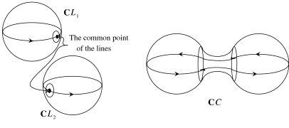
First, consider the simplest special case: a small perturbation of the union of two real lines. Denote the lines by $L_{1}$ and $L_{2}$ and the result by $C$. As we saw above, $\mathbb{C}L_{i}$ and $\mathbb{C}C$ are homeomorphic to $S^{2}$. The spheres $\mathbb{C}L_{1}$ and $\mathbb{C}L_{2}$ intersect each other at a single point. By the complex version of the implicit function theorem, $\mathbb{C}C$ approximates $\mathbb{C}L_{1}\cup\mathbb{C}L_{2}$ outside a neighborhood $U_{0}$ of this point in the sense that $\mathbb{C}C\smallsetminus U_{0}$ is a section of a tulubular neighborhood $U_{1}$ of $(\mathbb{C}L_{1}\cup\mathbb{C}L_{1})\smallsetminus U_{0}$, cf. 1.5.A. Thus $\mathbb{C}C$ may be presented as the union of two discs and a part contained in a small neighborhood of $\mathbb{C}L_{1}\cap\mathbb{C}L_{2}$. Since the whole $\mathbb{C}C$ is homeomorphic to $S^{2}$ and the complement of two disjoint discs embedded into $S^{2}$ is homeomorphic to the annulus, the third part of $\mathbb{C}C$ is an annulus. The discs are the complements of a neighborhood of $\mathbb{C}L_{1}\cap\mathbb{C}L_{2}$ in $\mathbb{C}L_{1}$ and $\mathbb{C}L_{2}$, respectively, slightly perturbed in $\mathbb{C}P^{2}$, and the annulus connects the discs through the neighborhood $U_{0}$ of $\mathbb{C}L_{1}\cap\mathbb{C}L_{2}$.
This is the complex view of the picture. Up to this point it does not matter whether the curves are defined by real equations or not.
To relate this to the real view presented in Section 1.5, one needs to describe the position of the real parts of the curves in their complexifications and the action of $conj$. It can be recovered by rough topological agruments. The whole complex picture above is invariant under $conj$. This means that the intersection point of $\mathbb{C}L_{1}$ and $\mathbb{C}L_{2}$ is real, its neighborhood $U_{0}$ can be chosen to be invariant under $conj$. Thus each half of $\mathbb{C}C$ is presented as the union of two half-discs and a half of the annulus: the half-discs approximate the halves of $\mathbb{C}L_{1}$ and $\mathbb{C}L_{2}$ and a half of annulus is contained in $U_{0}$. See Figure 15.
This is almost complete description. It misses only one point: one has to specify which half-discs are connected with each other by a half-annulus.
First, observe, that the halves of the complex point set of any curve of type I can be distinguished by the orientations of the real part. Each of the halves has the canonical orientation defined by the complex structure, and this orientation induces an orientation on the boundary of the half. This is one of the complex orientations. The other complex orientation comes from the other half. Hence the halves of the complexification are in one-to-one correspondence to the complex orientations.
Now we have an easy answer to the question above. The halves of $\mathbb{C}L_{i}$ which are connected with each other after the perturbation correspond to the complex orientations of $\mathbb{R}L_{i}$ which agree with some orientation of $\mathbb{R}C$. Indeed, the perturbed union $C$ of the lines $L_{i}$ is a curve of type I (since this is a nonempty conic, see Section 2.2). Each orientation of its real part $\mathbb{R}C$ is a complex orientation. Choose one of the orientations. It is induced by the canonical orientation of a half of the complex point set $\mathbb{C}C$. Its restriction to the part of the $\mathbb{R}C$ obtained from $\mathbb{R}L_{i}$ is induced by the orientation of the corresponding part of this half.
The union of two lines can be perturbed in two different ways. On the other hand, there are two ways to connect the halves of their complexifications. It is easy to see that different connections correspond to different perturbations. See Figure 16.

The special classical small perturbation considered above is a key for understanding what happens in the complex domain at an arbitrary classical small perturbation. First, look at the complex picture, forgetting about the real part. Take a plane projective curve, which has only nondegenerate double points. Near such a point it is organized as a union of two lines intersecting at the point. This means that there are a neighborhood $U$ of the point in $\mathbb{C}P^{2}$ and a diffeomorphism of $U$ onto $\mathbb{C}^{2}$ mapping the intersection of $U$ and the curve onto a union of two complex lines, which meet each other in 0. This follows from the complex version of the Morse lemma. By the same Morse lemma, near each double point the classical small perturbation is organized as a small perturbation of the union of two lines: the union of two transversal disks is replaced by an annulus.
For example, take the union of $m$ projective lines, no three of which have a common point. Its complex point set is the union of $m$ copies of $S^{2}$ such that any two of them have exactly one common point. A perturbation can be thought of as removal from each sphere $m-1$ disjoint discs and insertion $\frac{m(m-1)}{2}$ tubes connecting the boundary circles of the disks removed. The result is orientable (since it is a complex manifold). It is easy to realize that this is a sphere with $\frac{(m-1)(m-2)}{2}$ handles. One may prove this counting the Euler characteristic, but it may be seen directly: first, by inserting the tubes which join one of the lines with all other lines we get a sphere, then each additional tube gives rise to a handle. The number of these handles is
| $\left(\begin{matrix}m-1\\ 2\end{matrix}\right)=\frac{(m-1)(m-2)}{2}.$ |
By the way, this description shows that the complex point set of a nonsingular plane projective curve of degree $m$ realizes the same homology class as the union of $m$ complex projective lines: the $m$-fold generator of $H_{2}(\mathbb{C}P^{2})(=\mathbb{Z})$.
Now let us try to figure out what happens with the complex schemes in an arbitrary classical small perturbation of real algebraic curves. The general case requirs some technique. Therefore we restrict ourselves to the following intermediate assertion.
2.3.A .
(Fiedler Rok-78, Section 3.7 and Marin Mar-80.) Let $A_{1},\,\dots,\,A_{s}$ be nonsingular curves of degrees $m_{1},\,\dots,\,m_{s}$ such that no three of them pass through the same point and $A_{i}$ intersects transversally $A_{j}$ in $m_{i}m_{j}$ real points for any $i$, $j$. Let $A$ be a nonsingular curve obtained by a classical small perturbation of the union $A_{1}\cup\dots A_{s}$. Then $A$ is of type I if and only if all $A_{i}$ are of type I and there exists an orientation of $\mathbb{R}A$ which agrees with some complex orientations of $A_{1},\,\dots,\,A_{s}$ (it means that the deformation turning $A_{1}\cup\dots A_{s}$ into $A$ brings the complex orientations of $A_{i}$ to the orientations of the corresponding pieces of $\mathbb{R}A$ induced by a single orientation of the whole $\mathbb{R}A$).
If it takes place, then the orientation of $\mathbb{R}A$ is one of the complex orientations of $A$.
Proof.
If some of $A_{i}$ is of type II, then it has a pair of complex conjugate imaginary points which can be connected by a path in $\mathbb{C}A_{i}\smallsetminus\mathbb{R}A_{i}$. Under the perturbation this pair of points and the path survive (being only slightly shifted), since they are far from the intersection where the real changes happen. Therefore $A$ in this case is also of type II.
Assume now that all $A_{i}$ are of type I. If $A$ is also of type I then a half of $\mathbb{C}A$ is obtained from halves of $\mathbb{C}A_{i}$ as in the case considered above. The orientation induced on $\mathbb{R}A$ by the orientation of the half agrees with orientations induced from the halves of the corresponding pieces. Thus a complex orietation of $A$ agrees with complex orientations of $A_{i}$’s.
Again assume that all $A_{i}$ are of type I. Let some complex orientations of $A_{i}$ agree with a single orientation of $\mathbb{R}A$. As it follows from the Morse Lemma, at each intersection point the perturbation is organized as the model perturbation considered above. Thus the halves of $\mathbb{C}A_{i}$’s defining the complex orientations are connected. It cannot happen that some of the halves will be connected by a chain of halves to its image under $conj$. But that would be the only chance to get a curve of type II, since in a curve of type II each imaginary point can be connected with its image under $conj$ by a path disjoint from the real part. $\square$


2.4. Further Examples
Although Theorem 2.3.A describes only a very special class of classical small perturbations (namely perturbations of unions of nonsingular curves intersecting only in real points), it is enough for all constructions considered in Section 1. In Figures 17, 18, 19, 20, 21, 22 and 23 I reproduce the constructions of Figures 2, 3, 4, 6, 7, 10 and 11, enhancing them with complex orientations if the curve is of type I.
2.5. Digression: Oriented Topological Plane Curves
Consider an oriented topological plane curve, i. e. an oriented closed one-dimensional submanifold of the projective plane, cf. 1.2.
A pair of its ovals is said to be injective if one of the ovals is enveloped by the other.
An injective pair of ovals is said to be positive if the orientations of the ovals determined by the orientation of the entire curve are induced by an orientation of the annulus bounded by the ovals. Otherwise, the injective pair of ovals is said to be negative. See Figure 24. It is clear that the division of pairs of ovals into positive and negative pairs does not change if the orientation of the entire curve is reversed; thus, the injective pairs of ovals of a semioriented curve (and, in particular, a curve of type I) are divided into positive and negative. We let $\Pi^{+}$ denote the number of positive pairs, and $\Pi^{-}$ denote the number of negative pairs.

The ovals of an oriented curve one-sidedly embedded into $\mathbb{R}P^{2}$ can be divided into positive and negative. Namely, consider the Möbius strip which is obtained when the disk bounded by an oval is removed from $\mathbb{R}P^{2}$. If the integral homology classes which are realized in this strip by the oval and by the doubled one-sided component with the orientations determined by the orientation of the entire curve coincide, we say that the oval is negative, otherwise we say that the oval is positive. See Figure 25. In the case of a two-sided oriented curve, only the non-outer ovals can be divided into positive and negative. Namely, a non-outer oval is said to be positive if it forms a positive pair with the outer oval which envelops it; otherwise, it is said to be negative. As in the case of pairs, if the orientation of the curve is reversed, the division of ovals into positive and negative ones does not change. Let $\Lambda^{+}$ denote the number of positive ovals on a curve, and let $\Lambda^{-}$ denote the number of negative ones.

To describe a semioriented topological plane curve (up to homeomorphism of the projective plane) we need to enhance the coding system introduced in 1.2. The symbols representing positive ovals will be equipped with a superscript $+$, the symbols representing negative ovals, with a superscript $-$. This kind of code of a semioriented curve is complete in the following sense: for any two semioriented curves with the same code there exists a homeomorphism of $\mathbb{R}P^{2}$, which maps one of them to the other preserving semiorientations.
To describe the complex scheme of a curve of degree $m$ we will use, in the case of type I, the scheme of the kind described here, for its complex semiorientation, equipped with subscript I and superscript $m$ and, in the case of type II, the notation used for the real scheme, but equipped with subscript II and superscript $m$.
It is easy to check, that the coding of this kind of the complex scheme of a plane projective real algebraic curve describes the union of $\mathbb{R}P^{2}$ and the complex point set of the curve up to a homeomorphism mapping $\mathbb{R}P^{2}$ to itself.
In these notations, the complex schemes of cubic curves shown in Figure 17 are $\langle J\rangle_{II}^{3}$ and $\langle J\amalg 1^{-}\rangle_{I}^{3}$.
The complex schemes of quartic curves realized in Figure 18 are $\langle 0\rangle_{II}^{4}$, $\langle 1\rangle_{II}^{4}$, $\langle 2\rangle_{II}^{4}$, $\langle 1\langle 1^{-}\rangle\rangle_{I}^{4}$, $\langle 3\rangle_{II}^{4}$, $\langle 4\rangle_{I}^{4}$.
The complex schemes of quintic curves realized in Figure 19 are $\langle J\rangle_{II}^{5}$, $\langle J\amalg 1\rangle_{II}^{5}$, $\langle J\amalg 2\rangle_{II}^{5}$, $\langle J\amalg 1^{-}\langle 1^{-}\rangle\rangle_{I}^{5}$, $\langle J\amalg 3\rangle_{II}^{5}$, $\langle J\amalg 4\rangle_{II}^{5}$, $\langle J\amalg 1^{+}\amalg 3^{-}\rangle_{I}^{5}$ $\langle J\amalg 5\rangle_{II}^{5}$, $\langle J\amalg 3^{+}\amalg^{-}\rangle_{I}^{5}$.
In fact, these lists of complex schemes contain all schemes of nonsingular algebraic curves for degrees 3 and 5 and all nonempty schemes for degree 4. To prove this, we need not only constructions, but also restrictions on complex schemes. In the next two sections restrictions sufficient for this will be provided.
2.6. The Simplest Restrictions on a Complex Scheme
To begin with, recall the following obvious restriction, which was used in Section 2.2.
2.6.A .
A curve with empty real point set is of type II.$\square$
The next theorem is in a sense dual to 2.6.A.
2.6.B .
An M-curve is of type I.
Proof.
Let $A$ be an M-curve of degree $m$. Then $\mathbb{R}A$ is the union of
| $\frac{(m-1)(m-2)}{2}+1$ |
disjoint circles lying on $\mathbb{C}A$, which is a sphere with $\frac{(m-1)(m-2)}{2}$ handles. That many disjoint circles necessarily divide a sphere with $\frac{(m-1)(m-2)}{2}$ handles. Indeed, cut $\mathbb{C}A$ along $\mathbb{R}A$. The Euler characteristic of a surface has not changed. It equals
| $2-2\left(\frac{(m-1)(m-2)}{2}\right)=2-(m-1)(m-2).$ |
Then cap each boundary circle with a disk. Each component of $\mathbb{R}A$ gives rise to 2 boundary circles. Therefore the number of the boundary circles is $(m-1)(m-2)+2$. The surface which is obtained has Euler characteristic $2-(m-1)(m-2)+(m-1)(m-2)+2=4$. However, there is no connected closed surface with Euler characteristic 4. (A connected closed oriented surface is a sphere with $g$ handles for some $g\geq 0$; it has Euler characteristic $2-2g\leq 2$.) $\square$
2.6.C Klein’s Congruence (see Kle-22, page 172).
If $A$ is a curve of type I of degree $m$ with $l$ ovals, then $l\equiv[\frac{m}{2}]\mod 2$.
Proof.
Consider a half of $\mathbb{C}A$ bounded by $\mathbb{R}A$. Its Euler characteristic equals the half of the Euler characteristic of $\mathbb{C}A$, i.e. $1-\frac{(m-1)(m-2)}{2}$. Cap the boundary components of the half with disjoint disks. This increases the Euler characteristics by the number of components of $\mathbb{R}A$. In the case of even degree $m=2k$, the Euler characteristic of the result is $1-(2k-1)(k-1)+l\equiv k+l\mod 2$. In the case of odd degree $m=2k+1$, it is $1-k(2k-1)+l\equiv k+l\mod 2$. In both cases the Euler characteristic should be even, since the surface is closed orientable and connected (i.e. sphere with handles). Thus in both cases $k\equiv l\mod 2$, where $k=[m/2]$. $\square$
2.6.D A Nest of the Maximal Depth (see Rok-78, 3.6).
A real scheme of degree $m$ containing a nest of depth $k=[m/2]$ is of type I.
Such a scheme exists and is unique for any $m$ (for even $m$ it is just the nest, for odd $m$ it consists of the nest and the one-sided component). To realize the scheme, perturb the union of $k$ concentric circles and, in the case of odd $m$, a line disjoint from the circles. The uniqueness was proved in 1.3, see 1.3.C.
I preface the proof of 2.6.D with a construction interesting for its own. It provides a kind of window through which one can take a look at the imaginary part of $\mathbb{C}P^{2}$.
As we know (see Section 2.2), the complex point set of a real line is divided by its real point set into two halves, which are in a natural one-to-one correspondence with the orientations of the real line. The set of all real lines on the projective plane is the real point set of the dual projective plane. The halves of lines comprise a two-dimensional sphere covering this projective plane. An especially clear picture of these identifications appears, if one identifies real lines on the projective plane with real planes in $\mathbb{R}^{3}$ containing 0. A half of a line is interpreted as the corresponding plane with orientation. An oriented plane corresponds to its positive unit normal vector, which is nothing but a point of $S^{2}$. The complex conjugation $conj$ maps a half of a real line to the other half of the same line. It corresponds to the reversing of the orientation, which, in turn, corresponds to the antipodal involution $S^{2}\to S^{2}:x\mapsto-x$.
There is a unique real line passing through any imaginary point of $\mathbb{C}P^{2}$. To construct such a line, connect the point with the conjugate one. The connecting line is unique since a pair of distinct points determines a line, and this line is real, since it coincides with its image under $conj$.
Consequently, there is a unique half of a real line containing an imaginary point of $\mathbb{C}P^{2}$. This construction determines a fibration $p:\mathbb{C}P^{2}\smallsetminus\mathbb{R}P^{2}\to S^{2}$. The fibres of $p$ are the halves of real lines. Note that conjugate points of $\mathbb{C}P^{2}\smallsetminus\mathbb{R}P^{2}$ are mapped to antipodal points of $S^{2}$.
Proof of 2.6.D.
Let $A$ be a real projective curve of degree $m$ with a nest of depth $[m/2]$. Choose a point $P\in\mathbb{R}P^{2}$ from the domain encircled by the interior oval of the nest. Consider the great circle of $S^{2}$ consisting of halves of real lines which pass through $P$. Since each line passing through $P$ intersects $\mathbb{R}A$ in $m$ points, it cannot intersect $\mathbb{C}A\smallsetminus\mathbb{R}A$. Therefore the great circle has no common point with the image of $\mathbb{C}A\smallsetminus\mathbb{R}A$ under $p:\mathbb{C}P^{2}\smallsetminus\mathbb{R}P^{2}\to S^{2}$. But the image contains, together with any of its points, the antipodal point. Therefore it cannot be connected, and $\mathbb{C}A\smallsetminus\mathbb{R}A$ cannot be connected, too. $\square$
2.7. Rokhlin’s Complex Orientation Formula
Now we shall consider a powerful restriction on a complex orientation of a curve of type I. It is powerful enough to imply restrictions even on real schemes of type I. The first version of this restriction was published in 1974, see Rok-74. There Rokhlin considered only the case of an algebraic M-curve of even degree. In Mis-75 Mishachev considered the case of an algebraic M-curve of odd degree. For an arbitrary nonsingular algebraic curve of type I, it was formulated by Rokhlin Rok-78 in 1978. The proofs from Rok-74 and Mis-75 work in this general case. The only reason to restrict the main formulations in these early papers to M-curves was the traditional viewpoint on the subject of the topology of real plane algebraic curves.
Here are Rokhlin’s formulations from Rok-78.
2.7.A Rokhlin Formula.
If the degree $m$ is even and the curve is of type I, then
| $2(\Pi^{+}-\Pi^{-})=l-\frac{m^{2}}{4}.$ |
2.7.B Rokhlin-Mishachev Formula.
If $m$ is odd and the curve is of type I, then
| $\Lambda^{+}-\Lambda^{-}+2(\Pi^{+}-\Pi^{-})=l-\frac{m^{2}-1}{4}.$ |
Theorems 2.7.A and 2.7.B can be united into a single formulation. This requires, however, two preliminary definitions.
First, given an oriented topological curve $C$ on $\mathbb{R}P^{2}$, for any point $x$ of its complement, there is the index $i_{C}(x)$ of the point with respect to the curve. It is a nonnegative integer defined as follows. Draw a line $L$ on $\mathbb{R}P^{2}$ through $x$ transversal to $C$. Equip it with a normal vector field vanishing only at $x$. For such a vector field, one may take the velocity field of a rotation of the line around $x$. At each intersection point of $L$ and $C$ there are two directions transversal to $L$: the direction of the vector belonging to the normal vector field and the direction defined by the local orientation of $C$ at the point. Denote the number of intersection points where the directions are faced to the same side of $L$ by $i_{+}$ and the number of intersection points where the directions are faced to the opposite sides of $L$ by $i_{-}$. Then put $i_{C}(x)=|i_{+}-i_{-}|/2$.55Division by 2 appears here to make this notion closer to the well-known notion for an affine plane curve. In the definition for affine situation one uses a ray instead of entire line. In the projective situation there is no natural way to divide a line into two rays, but we still have an opportunity to divide the result by 2. Another distinction from the affine situation is that there the index may be negative. It is related to the fact that the affine plane is orientable, while the projective plane is not. It is easy to check that $i_{C}(x)$ is well defined: it depends neither on the choice of $L$, nor on the choice of the normal vector field. It does not change under reversing of the orientation of $C$. Thus for any nonsingular curve $A$ of type I on the complement $\mathbb{R}P^{2}\smallsetminus\mathbb{R}A$, one has well defined function $i_{\mathbb{R}A}$.
The second prerequisite notion is a sort of unusual integration: an integration with respect to the Euler characteristic, in which the Euler characteristic plays the role of a measure. It is well known that the Euler characteristic shares an important property of measures: it is additive in the sense that for any sets $A$, $B$ such that the Euler characteristics $\chi A$, $\chi B$, $\chi(A\cap B)$ and $\chi(A\cup B)$ are defined,
| $\chi(A\cup B)=\chi(A)+\chi(B)-\chi(A\cap B).$ |
However, the Euler characteristic is neither $\sigma$-additive, nor positive. Thus the usual theory of integral cannot be applied to it. This can be done though if one restricts to a very narrow class of functions. Namely, to functions which are finite linear combinations of characteristic functions of sets belonging to some algebra of subsets of a topological space such that each element of the algebra has a well defined Euler characteristic. For a function $f=\sum_{i=1}^{r}\lambda_{i}\hbox{\rm\hbox to 0.0pt{1} {{\rm I}}}_{S_{i}}$ set
| $\int f(x)\,d\chi(x)=\sum_{i=1}^{r}\lambda_{i}\chi(S_{i}).$ |
For details and applications of that notion, see Vir-88.
Now we can unite 2.7.A and 2.7.B:
2.7.C Rokhlin Complex Orientation Formula.
If $A$ is a nonsingular real plane projective curve of type I and degree $m$ then
| $\int(i_{\mathbb{R}A}(x))^{2}\,d\chi(x)=\frac{m^{2}}{4}.$ |
Here I give a proof of 2.7.C, skipping the most complicated details. Take a curve $A$ of degree $m$ and type I. Let $\mathbb{C}A_{+}$ be its half bounded by $\mathbb{R}A$. It may be considered as a chain with integral coefficients. The boundary of this chain (which is $\mathbb{R}A$ equipped with the complex orientation) bounds in $\mathbb{R}P^{2}$ a chain $c$ with rational coefficients, since $H_{1}(\mathbb{R}P^{2};\,\mathbb{Q})=0$. In fact, in the case of even degree the chain can be taken with integral coefficients, but in the case of odd degree the coefficients are necessarily half-integers. The explicit form of $c$ may be given in terms of function $i_{\mathbb{R}A}$: it is a linear combination of the fundamental cycles of the components of $\mathbb{R}P^{2}\smallsetminus\mathbb{R}A$ with coefficients equal to the values of $i_{\mathbb{R}A}$ on the components (taken with appropriate orientations).
Now take the cycle $[\mathbb{C}A_{+}]-c$ and its image under $conj$, and calculate their intersection number in two ways.
First, it is easy to see that the homology class $\xi$ of $[\mathbb{C}A_{+}]-c$ is equal to $$\frac{1}{2}[\mathbb{C}A]=\frac{m}{2}[\mathbb{C}P^{1}]\in H_{2}(\mathbb{C}P^{2} ;\,\mathbb{Q})$$ Indeed, $$[\mathbb{C}A_{+}]-c-conj([\mathbb{C}A_{+}]-c)=[\mathbb{C}A]+c-conj(c)=[\mathbb {C}A]$$, and therefore $$\xi-conj_{*}(\xi)=[\mathbb{C}A]=m[\mathbb{C}P^{1}]\in H_{2}(\mathbb{C}P^{2}).$$ On the other hand, $conj$ acts in $H_{2}(\mathbb{C}P^{2})$ as multiplication by $-1$, and hence $\xi-conj_{*}(\xi)=2\xi=m[\mathbb{C}P^{1}]$. Therefore $\xi\circ conj_{*}(\xi)=-(\frac{m}{2})^{2}$.
Second, one may calculate the same intersection number geometrically: moving the cycles into a general position and counting the local intersection numbers. I will perturb the cycle $[\mathbb{C}A_{+}]-c$. First, choose a smooth tangent vector field $V$ on $\mathbb{R}P^{2}$ such that it has only nondegenerate singular points, the singular points are outside $\mathbb{R}A$, and on $\mathbb{R}A$ the field is tangent to $\mathbb{R}A$ and directed according to the complex orientation of $A$ which comes from $\mathbb{C}A_{+}$. The latter means that at any point $x\in\mathbb{R}A$ the vector $\sqrt{-1}V(x)$ is directed inside $\mathbb{C}A_{+}$ (the multiplication by $\sqrt{-1}$ makes a real vector normal to the real plane and lieves any vector tangent to $\mathbb{R}A$ tangent to $\mathbb{C}A$). Now shift $\mathbb{R}A$ inside $\mathbb{C}A_{+}$ along $\sqrt{-1}V$ and extend this shift to a shift of the whole chain $c$ along $\sqrt{-1}V$. Let $c^{\prime}$ denote the result of the shift of $c$ and $h$ denote the part of $\mathbb{C}A_{+}$ which was not swept during the shift. The cycle $[h]-c^{\prime}$ represents the same homology class $\xi$ as $[\mathbb{C}A_{+}]-c$, and we can use it to calculate the intersection number $\xi\circ conj_{*}(\xi)$. The cycles $[h]-c^{\prime}$ and $conj([\mathbb{C}A_{+}]-c)$ intersect only at singular points of $V$. At a singular point $x$ they are smooth transversal two-dimensional submanifolds, each taken with multiplicity $-i_{\mathbb{R}A}(x)$. The local intersection number at $x$ is equal to $(i_{\mathbb{R}A}(x))^{2}$ multiplied by the local intersection number of the submanifolds supporting the cycles. The latter is equal to the index of the vector field $V$ at $x$ multiplied by $-1$.
I omit the proof of the latter statement. It is nothing but a straightforward checking that multiplication by $\sqrt{-1}$ induces isomorphism between tangent and normal fibrations of $\mathbb{R}A$ in $\mathbb{C}A$ reversing orientation.
Now recall that the sum of indices of a vector field tangent to the boundary of a compact manifold is equal to the Euler characteristic of the manifold. Therefore the input of singular points lying in a connected component of $\mathbb{R}P^{2}\smallsetminus\mathbb{R}A$ is equal to the Euler characteristic of the component multiplied by $-(i_{\mathbb{R}A}(x))^{2}$ for any point $x$ of the component. Summation over all connected components of $\mathbb{R}P^{2}\smallsetminus\mathbb{R}A$ gives $-\int(i_{\mathbb{R}A}(x))^{2}\,d\chi(x)$. Its equality to the result of the first calculation is the statement of 2.7.C.$\square$
2.7.D Corollary 1. Arnold Congruence.
For a curve of an even degree $m=2k$ and type I
| $p-n\equiv k^{2}\mod 4.$ |
Proof.
Observe that in the case of an even degree $i_{\mathbb{R}A}(x)$ is even, iff $x\in\mathbb{R}P^{2}_{+}$. Therefore
| $(i_{\mathbb{R}A}(x))^{2}\equiv\begin{cases}0\mod 4,\text{ if }x\in\mathbb{R}P^ {2}_{+}\\ 1\mod 4,\text{ if }x\in\mathbb{R}P^{2}_{-}.\end{cases}$ |
Thus
| $\int_{\mathbb{R}P^{2}}(i_{\mathbb{R}A}(x))^{2}\,d\chi(x)\equiv\chi(\mathbb{R}P ^{2}_{+})\mod 4.$ |
Recall that $\chi(\mathbb{R}P^{2}_{+})=p-n$, see 1.11. Hence the left hand side of Rokhlin’s formula is $p-n$ modulo 4. The right hand side is $k^{2}$. $\square$
Denote the number of all injective pairs of ovals for a curve under consideration by $\Pi$.
2.7.E Corollary 2.
For any curve of an even degree $m=2k$ and type I with $l$ ovals
| $\Pi\geq\frac{1}{2}|l-k^{2}|.$ |
Proof.
By 2.7.A $\Pi^{+}-\Pi_{-}=\frac{1}{2}(l-k^{2})$. On the other hand, $\Pi=\Pi_{+}+\Pi_{-}\geq|\Pi_{+}-\Pi_{-}|$. $\square$
2.7.F Corollary 3.
For any curve of an odd degree $m=2k+1$ and type I with $l$ ovals
| $\Pi+l\geq\frac{1}{2}k(k+1).$ |
Proof.
Since $l=\Lambda_{+}+\Lambda_{-}$, the Rokhlin - Mishachev formula 2.7.B can be rewritten as follows:
| $\Lambda_{-}+\Pi_{-}-\Pi_{+}=\frac{1}{2}k(k+1).$ |
On the other hand, $\Pi\geq\Pi_{-}-\Pi_{+}$ and $l\geq\Lambda_{-}$. $\square$
2.8. Complex Schemes of Degree $\leq 5$
As it was promised in Section 2.5, we can prove now that only schemes realized in Figures 17, 18 and 19 are realizable by curves of degree 3, 4 and 5, respectively. For reader’s convinience, I present here a list of all these complex schemes in Table 5.
$m$ Complex schemes of nonsingular plane curves of degree $m$ 1 $\langle J\rangle^{1}_{I}$ 2 $\langle 1\rangle^{2}_{I}$ $\langle 0\rangle^{2}_{II}$ 3 $\langle J\amalg 1^{-}\rangle^{3}_{I}$ $\langle J\rangle^{3}_{II}$ 4 $\langle 4\rangle^{4}_{I}$ $\langle 3\rangle^{4}_{II}$ $\langle 1\langle 1^{-}\rangle\rangle^{4}_{I}$ $\langle 2\rangle^{4}_{II}$ $\langle 1\rangle^{4}_{II}$ $\langle 0\rangle^{4}_{II}$ 5 $J\amalg 3^{+}\amalg 3^{-}\rangle_{I}^{5}$ $\langle J\amalg 5\rangle^{5}_{II}$ $\langle J\amalg 1^{+}\amalg 3^{-}\rangle_{I}^{5}$ $\langle J\amalg 4\rangle^{5}_{II}$ $\langle J\amalg 3\rangle^{5}_{II}$ $\langle J\amalg 1^{-}\langle 1^{-}\rangle\rangle^{5}_{I}$ $\langle J\amalg 2\rangle^{5}_{II}$ $\langle J\amalg 1\rangle^{5}_{II}$ $\langle J\rangle^{5}_{II}$
Degree 3. By Harnack’s inequality, the number of components is at most 2. By 1.3.B a curve of degree 3 is one-sided, thereby the number of components is at least 1. In the case of 1 component the real scheme is $\langle J\rangle$, and the type is II by Klein’s congruence 2.6.C. In the case of 2 components the type is I by 2.6.B. The real scheme is $\langle J\amalg 1\rangle$. Thus we have 2 possible complex schemes: $\langle J\amalg 1^{-}\rangle_{I}^{3}$ (realized above) and $\langle J\amalg 1^{+}\rangle_{I}^{3}$. For the first one $\int(i_{\mathbb{R}A}(x))^{2}\,d\chi(x)=9/4$ and for the second $\int(i_{\mathbb{R}A}(x))^{2}\,d\chi(x)=1/4$. Since the right hand side of the complex orientation formula is $m^{2}/4$ and $m=3$, only the first possibility is realizable.$\square$
Degree 4. By Harnack’s inequality the number of components is at most 4. We know (see 1.4) that only real schemes $\langle 0\rangle$, $\langle 1\rangle$, $\langle 2\rangle$, $\langle 1\langle 1\rangle\rangle$, $\langle 3\rangle$ and $\langle 4\rangle$ are realized by nonsingular algebraic curves of degree 4. From Klein’s congruence 2.6.C it follows that the schemes $\langle 1\rangle$ and $\langle 3\rangle$ are of type II. The scheme $\langle 0\rangle$ is of type II by 2.6.A. By 2.6.B $\langle 4\rangle$ is of type I.
The scheme $\langle 2\rangle$ is of type II, since it admits no orientation satisfying the complex orientation formula. In fact, for any orientation $\int(i_{\mathbb{R}A}(x))^{2}\,d\chi(x)=2$ while the right hand side is $m^{2}/4=4$.
By 2.6.D the scheme $\langle 1\langle 1\rangle\rangle$ is of type I. A calculation similar to the calculation above on the scheme $\langle 2\rangle$, shows that only one of the two semiorientations of the scheme $\langle 1\langle 1\rangle\rangle$ satisfies the complex orientation formula. Namely, $\langle 1\langle 1^{-}\rangle\rangle$. It was realized in Figure 18.
Degree 5. By Harnack’s inequality the number of components is at most 7. We know (see 1.4) that only real schemes $\langle J\rangle$, $\langle J\amalg 1\rangle$, $\langle J\amalg 2\rangle$, $\langle J\amalg 1\langle 1\rangle\rangle$, $\langle J\amalg 3\rangle$, $\langle J\amalg 4\rangle$, $\langle J\amalg 5\rangle$, $\langle J\amalg 6\rangle$ are realized by nonsingular algebraic curves of degree 5. From Klein’s congruence 2.6.C it follows that the schemes $\langle J\amalg 1\rangle$, $\langle J\amalg 3\rangle$, $\langle J\amalg 5\rangle$ are of type II. By 2.7.F $\langle J\rangle$ and $\langle J\amalg 2\rangle$ are of type II.
By 2.6.B $\langle J\amalg 6\rangle$ is of type I. The complex orientation formula gives the value of $\Lambda_{-}$ (cf. Proof of 2.7.F): $\Lambda_{-}=\frac{1}{2}k(k+1)=3$. This determines the complex scheme. It is $\langle J\amalg 3^{-}\amalg 3^{+}\rangle_{I}^{5}$.
By 2.6.D $\langle J\amalg 1\langle 1\rangle\rangle$ is of type I. The complex orientation formula allows only the semiorientation with $\Lambda_{-}=2$. Cf. Figure 19.
The real scheme $\langle J\amalg 4\rangle$ is of indefinite type, as follows from the construction shown in Figure 19. In the case of type I only one semiorientation is allowed by the the complex orientation formula. It is $\langle J\amalg 3^{-}\amalg 1^{+}\rangle_{I}^{5}$.
Exercises
2.1 Prove that for any two semioriented curves with the same code (of the kind introduced in 3.7) there exists a homeomorphism of $\mathbb{R}P^{2}$ which maps one of them to another preserving semiorientations.
2.2 Prove that for any two curves $A_{1}$, $A_{2}$ with the same code of their complex schemes (see Subsection 2.5) there exists a homeomorphism $\mathbb{C}A_{1}\cup\mathbb{R}P^{2}\to\mathbb{C}A_{2}\cup\mathbb{R}P^{2}$ commuting with $conj$.
2.3 Deduce 2.7.A and 2.7.B from 2.7.C and, vise versa, 2.7.C from 2.7.A and 2.7.B.
3. The Topological Point of View on Prohibitions
3.1. Flexible Curves
In Section 1 all prohibitions were deduced from the Bézout Theorem. In Section 2 many proofs were purely topological. A straightforward analysis shows that the proofs of all prohibitions are based on a small number of basic properties of the complexification of a nonsingular plane projective algebraic curve. It is not difficult to list all these properties of such a curve $A$:
-
(1)
Bézout’s theorem;
-
(2)
$\mathbb{C}A$ realizes the class $m[\mathbb{C}P^{1}]\in H_{2}(\mathbb{C}P^{2})$;
-
(3)
$\mathbb{C}A$ is homeomorphic to a sphere with $(m-1)(m-2)/2$ handles;
-
(4)
$conj(\mathbb{C}A)=conj$;
-
(5)
the tangent plane to $\mathbb{C}A$ at a point $x\in\mathbb{R}A$ is the complexification of the tangent line of $\mathbb{R}A$ at $x$.
The last four are rough topological properties. Bézout’s theorem occupies a special position. If we assume that some surface smoothly embedded into $\mathbb{C}P^{2}$ intersects the complex point set of any algebraic curve as, according to Bézout’s theorem, the complex point set of an algebraic curve, then this surface is the complex point set of an algebraic curve. Thus the Bézout theorem is completely responsible for the whole set of properties of algebraic curves. On the other hand, its usage in obtaining prohibitions involves a construction of auxiliary curves, which may be very subtle.
Therefore, along with algebraic curves, it is useful to consider objects which imitate them topologically.
An oriented smooth closed connected two-dimensional submanifold $S$ of the complex projective plane $\mathbb{C}P^{2}$ is called a flexible curve of degree $m$ if:
-
(i)ii
$S$ realizes $m[\mathbb{C}P^{1}]\in H_{2}(\mathbb{C}P^{2})$;
-
(ii)i
the genus of $S$ is equal to $(m-1)(m-2)/2$;
-
(iii)
$conj(S)=S$;
-
(iv)
the field of planes tangent to $S$ on $S\cap\mathbb{R}P^{2}$ can be deformed in the class of planes invariant under $conj$ into the field of (complex) lines in $\mathbb{C}P^{2}$ which are tangent to $S\cap\mathbb{R}P^{2}$.
A flexible curve $S$ intersects $\mathbb{R}P^{2}$ in a smooth one-dimensional submanifold, which is called the real part of $S$ and denoted by $\mathbb{R}S$. Obviously, the set of complex points of a nonsingular algebraic curve of degree $m$ is a flexible curve of degree $m$. Everything said in Section 2.1 about algebraic curves and their (real and complex) schemes carries over without any changes to the case of flexible curves. We say that a prohibition on the schemes of curves of degree $m$ comes from topology if it can be proved for the schemes of flexible curves of degree $m$. The known classification of schemes of degree $\leq 6$ can be obtained using only the prohibitions that come from topology. In other words, for $m\leq 6$ all prohibitions come from topology.
3.2. The Most Elementary Prohibitions on Real Topology of a Flexible Curve
The simplest prohibitions are not related to the position of $\mathbb{R}S$ in $\mathbb{R}P^{2}$, but deal with the following purely topological situation: a surface $S$, which is homeomorphic to a sphere with $g$ ($=(m-1)(m-2)/2$) handles, and an involution $c$ ($=conj$) of $S$ reversing orientation with fixed point set $F$ ($=\mathbb{R}S$).
The most important of these prohibitions is Harnack’s inequality. Recall that it is
| $L\leq\frac{(m-1)(m-2)}{2}+1,$ |
where $L$ is the number of connected components of the real part a curve and $m$ is its degree. Certainly, this formulation given in Section 1.3 can be better adapted to the context of flexible curves. The number $\frac{(m-1)(m-2)}{2}$ is nothing but the genus. Therefore the Harnack inequality follows from the following theorem.
3.2.A .
For a reversing orientation involution $c:S\to S$ of a sphere $S$ with $g$ handles, the number $L$ of connected components of the fixed point set $F$ is at most $g+1$.
In turn, 3.2.A can be deduced from the following purely topological theorem on involutions:
3.2.B Smith-Floyd Theorem.
For any involution $i$ of a topological space $X$,
| $\dim_{\mathbb{Z}_{2}}H_{*}(fix(i);\,\mathbb{Z}_{2})\leq\dim_{\mathbb{Z}_{2}}H_ {*}(X;\,\mathbb{Z}_{2}).$ |
This theorem is one of the most famous results of the Smith theory. It is deduced from the basic facts on equivariant homology of involution, see, e. g., Bre-72, Chapter 3.
Theorem 3.2.A follows from 3.2.B, since
| $\dim_{\mathbb{Z}_{2}}H_{*}(S;\,\mathbb{Z}_{2})=2+2g,$ |
and
| $\dim_{\mathbb{Z}_{2}}H_{*}(F;\,\mathbb{Z}_{2})=2L.$ |
Smith - Floyd Theorem can be applied to high-dimensional situation, too. See Sections 5.3 and LABEL:s15.1d. In the one-dimensional case, which we deal with here, Theorem 3.2.B is easy to prove without any homology tool, like the Smith theory. Namely, consider the orbit space $S/c$ of the involution. It is a connected surface with boundary. The boundary is the image of the fixed point set. The Euler characteristic of the orbit space is equal to the half of the Euler characteristic of $S$, i.e. it is $\frac{2-2g}{2}=1-g$. Cap each boundary circle with a disk. The result is a closed connected surface with Euler characteristic $1-g+L$. On the other hand, as it is well known, the Euler characteristic of a connected closed surface is at most 2. (Remind that such a surface is homeomorphic either to the sphere, which has Euler characteristic 2, or the sphere with $h$ handles, whose Euler characteristic is $2-2h$, or sphere with $h$ Möbius strips having Euler characteristic $2-h$.) Therefore $1-g+L\leq 2$, and $L\leq g+1$.$\square$
These arguments contain more than just a proof of 2.3.A. In particular, they imply that
3.2.C .
In the case of an M-curve (i.e., if $L=g+1$) and only in this case, the orbit space is a sphere with holes.
Similarly, in the case of an $(M-1)$-curve, the orbit space is homeomorphic to the projective plane with holes.
If $F$ separates $S$ (i.e., $S\smallsetminus F$ is not connected), the involution $c$ is said to be of type I, otherwise it is said to be of type II. The types correspond to the types of real algebraic curves (see Section 2.1).
Note that $F$ separates $S$ at most into two pieces. To prove this, we can use the same arguments as in a footnote in Section 2.1: the closure of tne union of a connected component of $S\smallsetminus F$ with its image under $c$ is open and close in $S$, but $S$ is connected.
3.2.D .
The orbit space $S/c$ is orientable if and only if $F$ separates $S$.
Proof.
Assume that $F$ separates $S$. Then the halves are homeomorphic, since the involution maps each of them homeomorphically onto the other one. Therefore, each of the halves is homeomorphic to the orbit space. The halves are orientable since the whole surface is.
On the other hand, if $F$ does not separate $S$, then one can connect a point of $S\smallsetminus F$ to its image under the involution by a path in the complement $S\smallsetminus F$. Such a path covers a loop in the orbit space. This is an orientation reversing loop, since the involution reverses orientation.$\square$
3.2.E (Cf. 2.6.C).
If the curve is of type I, then $L\equiv\left[\frac{m+1}{2}\right]\mod 2$.
Proof.
This theorem follows from 3.2.C and the calculation of the Euler characteristic of $S/c$ made in the proof of the Harnack inequality above. Namely, $\chi(S/c)=1-g$, but for any orientable connected surface with Euler characteristic $\chi$ and $L$ boundary components $\chi+L\equiv 0\mod 2$. Therefore $1-g+L\equiv 0\mod 2$. Since $g=(m-1)(m-2)/2\equiv\left[\frac{m-1}{2}\right]\mod 2$, we obtain $1-\left[\frac{m-1}{2}\right]+L\equiv 0\mod 2$ which is equivalent to the desired congruence.$\square$
3.2.F (Cf. 2.6.B).
Any M-curve is of type I.
Proof.
By 3.2.C, in the case of M-curve the orbit space $S/c$ is homeomorphic to a sphere with holes. In particular, it is orientable. By 3.2.D, this implies that $F$ separates $S$. $\square$
Now consider the simplest prohibition involving the placement of the real part of the flexible curve in the projective plane.
3.2.G .
The real part of a flexible curve is one-sided if and only if the degree is odd.
Proof.
The proof of 3.2.G coincides basically with the proof of the same statement for algebraic curves. One has to consider a real projective line transversal to the flexible curve and calculate the intersection number of the complexification of this line and the lfexible curve. On one hand, it is equal to the degree of the flexible curve. On the other hand, the intersection points in $\mathbb{C}P^{2}\smallsetminus\mathbb{R}P^{2}$ give rise to an even contribution to the intersection number.$\square$
Rokhlin’s complex orientation formula also comes from topology. The proof presented in Section 2.7 works for a flexible curve.
At this point I want to break a textbook style exposition. Escaping a detailed exposition of prohibitions, I switch to a survey.
In the next two sections, the current state of prohibitions on the topology of a flexible curve of a given degree is outlined. (Recall that all formulations of this sort are automatically valid for real projective algebraic plane curves of the same degree.) After the survey a light outline of some proofs is proposed. It is included just to convey a general impression, rather than for more serious purposes. For complete proofs, see the surveys Wil-78, Rok-78, Arn-79, Kha-78, Kha-86, Vir-86 and the papers cited there.
3.3. A Survey of Prohibitions on the Real Schemes Which Come from Topology
In this section I list all prohibitions on the real scheme of a flexible curve of degree $m$ that I am aware of, including the ones already referred to above, but excluding prohibitions which follow from the other prohibitions given here or from the prohibitions on the complex schemes which are given in the next section.
3.3.A .
A curve is one-sided if and only if it has odd degree.
This fact was given before as a corollary of Bézout’s theorem (see Section 1.3) and proved for flexible curves in Section 3.2 (Theorem 3.2.G).
3.3.B Harnack’s Inequality.
The number of components of the set of real points of a curve of degree $m$ is at most $\frac{(m-1)(m-2)}{2}+1$.
Harnack’s inequality is undoubtedly the best known and most important prohibition. It can also be deduced from Bézout’s theorem (cf. Section 1.3) and was proved for flexible curves in Section 3.2 (Theorem 3.2.A).
In prohibitions 3.3.C–3.3.P the degree $m$ of the curve is even: $m=2k$.
Extremal Properties of Harnack’s Inequality
3.3.C Gudkov-Rokhlin Congruence.
In the case of an M-curve (i.e., if $p+n=(m-1)(m-2)/2+1$),
| $p-n\equiv k^{2}\quad\mod 8.$ |
3.3.D Gudkov-Krakhnov-Kharlamov Congruence.
In the case of an$(M-1)$-curve (i.e., if $p+n=\frac{(m-1)(m-2)}{2}$),
| $p-n\equiv k^{2}\pm 1\quad\mod 8.$ |
The Euler characteristic of a component of the complement of a curve in $\mathbb{R}P^{2}$ is called the characteristic of the oval which bounds the component from outside. An oval with a positive characteristic is said to be elliptic, an oval with the zero characteristic is said to be parabolic and an oval with a negative characteristic is said to be hyperbolic.
3.3.E Fiedler’s Congruence.
If the curve is an M-curve, $m\equiv 4\mod 8$, and every even oval has an even characteristic, then
| $p-n\equiv-4\quad\mod 16.$ |
3.3.F Nikulin’s Congruence.
If the curve is an M-curve, $m\equiv 0\mod 8$, and the characteristic of every even oval is divisible by $2^{r}$, then
| (3) | $\displaystyle\text{ either }p-n\equiv$ | $\displaystyle 0\mod 2^{r+3},$ | ||
| (4) | $\displaystyle\text{or else }p-n=$ | $\displaystyle 4^{q}\chi,$ |
where $q\geq 2$ and $\chi\equiv 1\mod 2$.
3.3.G Nikulin’s Congruence.
If the curve is an M-curve, $m\equiv 2\mod 4$ and the characteristic of every odd oval is divisible by $2^{r}$, then
| $p-n\equiv 1\quad\mod 2^{r+3}.$ |
Denote the number of even ovals with positive characteristic by $p^{+}$, the number of even ovals with zero characteristic by $p^{0}$, and the number of even ovals with negative characteristic by $p^{-}$. Similarly define $n^{+},n^{0}$ and $n^{-}$ for the odd ovals; and let $l^{+},l^{0}$ and $l^{-}$ be the corresponding numbers for both even and odd ovals together.
Refined Petrovsky Inequalities
3.3.H .
$p-n^{-}\leq\frac{3k(k-1)}{2}+1$ .
3.3.I .
$n-p^{-}\leq\frac{3k(k-1)}{2}$ .
Refined Arnold Inequalities
3.3.J .
$p^{-}+p^{0}\leq\frac{(k-1)(k-2)}{2}+\frac{1+(-1)^{k}}{2}$ .
3.3.K .
$n^{-}+n^{0}\leq\frac{(k-1)(k-2)}{2}$ .
Extremal Properties of the Refined Arnold Inequalities
3.3.L .
If $k$ is even and $p^{-}+p^{0}=\frac{(k-1)(k-2)}{2}+1$, then $p^{-}=p^{+}=0$.
3.3.M .
If $k$ is odd and $n^{-}+n^{0}=\frac{(k-1)(k-2)}{2}$, then $n^{-}=n^{+}=0$ and there is only one outer oval at all.
Viro-Zvonilov Inequalities
Besides Harnack’s inequality, we know only one family of prohibition coming from topology which extends to real schemes of both even and odd degree. For proofs see VZ-92.
3.3.N Bound of the Number of Hyperbolic Ovals.
The number of components of the complement of a curve of odd degree $m$ that have a negative Euler characteristic does not exceed $\frac{(m-3)^{2}}{4}$. In particular, for any odd $m$
| $l^{-}\leq\frac{(m-3)^{2}}{4}.$ |
The latter inequality also holds true for even $m\neq 4$, but it follows from Arnold inequalities 3.3.J and 3.3.K.
3.3.O Bound of the Number of Nonempty Ovals.
If $h$ is a divisor of $m$ and a power of an odd prime, and if $m\neq 4$, then
| $l^{-}+l^{0}\leq\frac{(m-3)^{2}}{4}+\frac{m^{2}-h^{2}}{4h^{2}}.$ |
If $m$ is even, this inequality follows from 3.3.J–3.3.L.
3.3.P Extremal Property of the Viro-Zvonilov Inequality.
If
| $l^{-}+l^{0}=\frac{(m-3)^{2}}{4}+\frac{m^{2}-h^{2}}{4h^{2}},$ |
where $h$ is a divisor of $m$ and a power of an odd prime $p$, then there exist $\alpha_{1},\ldots,\alpha_{r}\in\mathbb{Z}_{p}$ and components $B_{1},\ldots,B_{r}$ of the complement $\mathbb{R}P^{2}\setminus\mathbb{R}A$ with $\chi(B_{1})=\cdots=\chi(B_{r})=0$, such that the boundary of the chain $\sum^{r}_{i=1}\alpha_{i}[B_{i}]\in C_{2}(\mathbb{R}P^{2};\mathbb{Z}_{p})$ is $[\mathbb{R}A]\in C_{1}(\mathbb{R}P^{2};\mathbb{Z}_{p})$.
3.4. Survey of Prohibitions on the Complex Schemes Which Come From Topology
Recall that $l$ denotes the total number of ovals on the curve. The following theorem is a reformulation of 3.2.E.
3.4.A See 2.6.A.
A curve with empty real point set is of type II.
3.4.B (See 2.6.C).
If the curve is of type I, then
| $l\equiv\left[\frac{m}{2}\right]\mod 2.$ |
3.4.C Rokhlin Complex Orientation Formula (see 2.7.C).
Let $A$ be a nonsingular curve of type I and degree $m$. Then
| $\int(i_{\mathbb{R}A}(x))^{2}\,d\chi(x)=\frac{m^{2}}{4}$ |
Extremal Properties of Harnack’s Inequality
3.4.D (Cf. 2.6.B).
Any M-curve is of type I.
3.4.E Kharlamov-Marin Congruence.
Any $(M-2)$-curve of even degree $m=2k$ with
| $p-n\equiv k^{2}+4\mod 8$ |
is of type I.
Extremal Properties of the Refined Arnold Inequalities
3.4.F .
If $m\equiv 0\mod 4$ and $p^{-}+p^{0}=\frac{(m-2)(m-4)}{8}+1$, then the curve is of type I.
3.4.G .
If $m\equiv 0\mod 4$ and $n^{-}+n^{0}=\frac{(m-2)(m-4)}{8}$, then the curve is of type I.
Extremal Properties of the Viro-Zvonilov Inequality
3.4.H .
Under the hypothesis of 3.3.P, the curve is of type I.
Congruences
3.4.I Nikulin-Fiedler Congruence.
If $m\equiv 0\mod 4$, the curve is of type I, and every even oval has even characteristic, then $p-n\equiv 0\mod 8$.
The next two congruences are included violating a general promise given at the beginning of the previous section. There I promised exclude prohibitions which follow from other prohibitions given here. The following two congruences are consequences of Rokhlin’s formula 3.4.C. The first of them was discovered long before 3.4.C. The second was overlooked by Rokhlin in Rok-74, where he even mistakenly proved that such a result cannot exist. Namely, Rokhlin proved that the complex orientation formula does not imply any result which would not follow from the prohibitions known by that time and could be formulated solely in terms of the real scheme. Slepian congruence 3.4.K for M-curves is the only counter-example to this Rokhlin’s statement. Slepian was Rokhlin’s student, he discovered a gap in Rokhlin’s arguments and deduced 3.4.K.
3.4.J Arnold Congruence (see 2.7.D).
If $m$ is even and the curve is of type I, then
| $p-n\equiv\frac{m^{2}}{4}\mod 4.$ |
3.4.K Slepian Congruence.
If $m$ is even, the curve is of type I, and every odd oval has even characteristic, then
| $p-n\equiv\frac{m^{2}}{4}\mod 8.$ |
Rokhlin Inequalities
Denote by $\pi$ and $\nu$ the number of even and odd nonempty ovals, respectively, bounding from the outside those components of the complement of the curve which have the property that each of the ovals bounding them from the inside envelops an odd number of other ovals.
3.4.L .
If the curve is of type I and $m\equiv 0\mod 4$, then
| $4\nu+p-n\leq\frac{(m-2)(m-4)}{2}+4.$ |
3.4.M .
If the curve is of type I and $m\equiv 2\mod 4$, then
| $4\pi+n-p\leq\frac{(m-2)(m-4)}{2}+3.$ |
3.5. Ideas of Some Proofs
Theorems formulated in 3.3 and 3.4 are very different in their profundity. The simplest of them were considered in Subsection 3.2.
Congruences
There are two different approaches to proving congruences. The first is due basically to Arnold Arn-71 and Rokhlin Rok-72. It is based on consideration of the intersection form of two-fold covering $Y$ of $\mathbb{C}P^{2}$ branched over the complex point set of the curve. The complex conjugation involution $conj:\mathbb{C}P^{2}\to\mathbb{C}P^{2}$ is lifted to $Y$ in two different ways, and the liftings induce involutions in $H_{2}(Y)$, which are isometries of the intersection form. One has to take an appropriate eigenspace of one of the liftings and consider the restriction of the intersection form to the eigenspace. The signature of this restriction can be calculated in terms of $p-n$. On the other hand, it is involved into some congruences of purely arithmetic nature relating it with the discriminant of the form and the value of the form on some of characteristic vectors. The latters can be calculated sometimes in terms of degree and the difference between the number of ovals and the genus of curve. Realizations of this scheme can be found in Arn-71 for 3.4.J, Rok-72 for 3.3.C, Kha-73 and GK-73 for 3.3.D, Nik-83 for 3.3.F, 3.3.G, 3.4.I and a weakened form of 3.3.E. In survey Wil-78 this method was used for proving 3.3.C, 3.3.D and 3.4.J.
The second approach is due to Marin Mar-80. It is based on application of the Rokhlin-Guillou-Marin congruence modulo 16 on characteristic surface in a 4-manifold, see GM-77. It is applied either to the surface in the quotient space $\mathbb{C}P^{2}/conj$ (diffeomorphic to $S^{4}$) made of the image of the flexible curve $S$ and a half of $\mathbb{R}P^{2}$ bounded by $\mathbb{R}S$ (as it is the case for proofs of 3.3.C, 3.3.D and 3.4.E in Mar-80), or to the surface in $\mathbb{C}P^{2}$ made of a half of $S$ and a half of $\mathbb{R}P^{2}$ (as it is the case for proofs of 3.3.E, 3.4.I and special cases of 3.3.F and 3.3.G in Fie-83).
The first approach was applied also in high-dimensional situations. The second approach worked better than the second one for curves on surfaces distinct from projective plane, see Mik-94. Both were used for singular curves KV-88.
Inequalities
Inequalities 3.3.H, 3.3.I, 3.3.J, 3.3.K, 3.4.J and 3.4.K are proved along the same scheme, originated by Arnold Arn-71. One constructs an auxiliary manifold, which is the two-fold covering of $\mathbb{C}P^{2}$ branched over $S$ in the case of 3.3.H, 3.3.I, 3.3.J and 3.3.K and the two-fold covering of $\mathbb{C}P^{2}/conj$ branched over the union of $S/conj$ and a half of $\mathbb{R}P^{2}$ in the case of 3.4.J and 3.4.K. Then preimages of some of the components of $\mathbb{R}P^{2}\smallsetminus\mathbb{R}S$ gives rise to cycles in this manifold. Those cycles define homology classes with special properties formulated in terms of their behavior with respect to the intersection form and the complex conjugation involutions. On the other hand, the numbers of homology classes with these properties are estimated. See Arn-71, Gud-74, Wil-78 and Rok-80.
3.6. Flexible Curves of Degrees $\leq 5$
In this subsection, I show that for degrees $\leq 5$ the prohibitions coming from topology allow the same set of complex schemes as all prohibitions. The set of complex schemes of algebraic curves of degrees $\leq 5$ was described in 2.8. In fact the same is true for degree 6 too. For degree greater than 6, it is not known, but there is no reason to believe that it is the case.
Degrees $\leq 3$. Theorems 3.3.A and the Harnack inequality 3.3.B prohibit all non realizable real schemes for degree $\leq 3$. To obtain the complete set of prohibitions for complex schemes of degrees $\leq 3$ one has to add the Klein congruence 3.4.B, 3.4.D and the complex orientation formula 3.4.C; cf. Section 2.8.
Degree 4. By the Arnold inequlity 3.3.K, a flexible curve of degree 4 cannot have a nest of depth 3. By the Arnold inequality 3.3.J, it has at most one nonempty positive oval, and if it has a nonempty oval then, by the extremal property 3.3.L of this inequality, the real scheme is $\langle 1\langle 1\rangle\rangle$. Together with 3.3.A and the Harnack inequality 3.3.B, this forms the complete set of prohibitions for real schemes of degree 4.
From the Klein congruence 3.4.B, it follows that the real schemes $\langle 1\rangle$ and $\langle 3\rangle$ are of type II. The empty real scheme $\langle 0\rangle$ is of type II by 3.4.A. By the extremal property 3.4.D of the Harnack inequality, $\langle 4\rangle$ is of type I. The real scheme $\langle 2\rangle$ is of type II by the complex orientation formula 3.4.C, cf. Section 2.8. By 3.4.F, the scheme $\langle 1\langle 1\rangle\rangle$ is of type I. By the complex orientation formula, it admits only the complex orientation $\langle 1\langle 1^{-}\rangle\rangle$.
Degree 5. By the Viro-Zvonilov inequality 3.3.O, a flexible curve of degree 5 can have at most one nonempty oval. By the extremal property of this inequality 3.3.P, if a flexible curve of degree 5 has a nonempty oval, then its real scheme is $\langle J\amalg 1\langle 1\rangle\rangle$. Together with 3.3.A and the Harnack inequality 3.3.B, this forms the complete set of prohibitions for real schemes of degree 5.
From the Klein congruence 3.4.B, it follows that the real schemes $\langle J\amalg 1\rangle$, $\langle J\amalg 3\rangle$, and $\langle J\amalg 5\rangle$ are of type II. From the complex orientation formula, one can deduce that the real schemes $\langle J\rangle$ and $\langle J\amalg 2\rangle$ are of type II, cf. 2.8. By the extremal property 3.4.D of the Harnack inequality, $\langle J\amalg 6\rangle$ is of type I. The complex orientation formula allows only one complex semiorientation for this scheme, namely $\langle J\amalg 3^{-}\amalg 3^{+}\rangle$. By the 3.4.H, the real scheme $\langle J\amalg 1\langle 1\rangle\rangle$ is of type I. The complex orientation formula allows only one complex semiorientation for this scheme, namely $\langle J\amalg 1^{-}\langle 1^{-}\rangle\rangle$, cf. 2.8. The real scheme $\langle J\amalg 4\rangle$ is of indefinite type (even for algebraic curves, see 2.8). In the case of type I, only one semiorientation is allowed by the the complex orientation formula. It is $\langle J\amalg 3^{-}\amalg 1^{+}\rangle$.
3.7. Sharpness of the Inequalities
The arsenal of constructions in Section 1 and the supply of curves constructed there, which are very modest from the point of view of classification problems, turn out to be quite rich if we are interested in the problem of sharpness of the inequalities in Section 3.3.
The Harnack curves of even degree $m$ with scheme
| $\langle(3m^{2}-6m)/8\amalg 1\langle m^{2}-6m+8)/8\rangle\rangle$ |
which were constructed in Section 1.6 (see also Section 1.9) not only show that Harnack’s inequality 3.3.B is the best possible, but also show the same for the refined Petrovsky inequality 3.3.H.
One of the simplest variants of Hilbert’s construction (see Section 1.10) leads to the construction of a series of M-curves of degree $m\equiv 2\mod 4$ with scheme $\left\langle\frac{(m-2)(m-4)}{8}\amalg 1\left\langle\frac{3m(m-2)}{8}\right \rangle\right\rangle$. This proves that the refined Petrovsky inequality 3.3.I for $m\equiv 2\mod 4$ is sharp. If $m\equiv 0\mod 4$, the methods of Section 1 do not show that this inequality is the best possible. This fact will be proved below in LABEL:s5.4s.
The refined Arnold inequality 3.3.J is best possible for any even $m$. If $m\equiv 2\mod 4$, this can be proved using the Wiman M-curves (see the end of Section 1.12). If $m\equiv 0\mod 4$, it follows using curves obtained from a modification of Wiman’s construction: the construction proceeds in exactly the same way, except that the opposite perturbation is taken, as a result of which one obtains a curve that can serve as the boundary of a tubular neighborhood of an M-curve of degree $m/2$.
The last construction (doubling), if applied to an M-curve of odd degree, shows that the refined Arnold inequality 3.3.K is the best possible for $m\equiv 2\mod 4$. If $m\equiv 0\mod 4$, almost nothing is known about sharpness of the inequality 3.3.K, except that for $m=8$ the right side can be lowered by 2.
3.8. Prohibitions not Proven for Flexible Curves
In conclusion of this section, let us come back to algebraic curves. We see that to a great extent the topology of their real point sets is determined by the properties which were included into the definition of flexible curves. In fact, it has not been proved that it is not determined by these properties completely. However some known prohibitions on topology of real algebraic curves have not been deduced from them.
As a rule, these prohibitions are hard to summarize, in the sense that it is difficult to state in full generality the results obtained by some particular method. To one extent or another, all of them are consequences of Bézout’s theorem.
Consider first the restrictions which follow directly from the Bézout theorem. To state them, we introduce the following notations. Denote by $h_{r}$ the maximum number of ovals occurring in a union of $\leq r$ nestings. Denote by $h^{\prime}_{r}$ the maximum number of ovals in a set of ovals contained in a union of $\leq r$ nests but not containing an oval which envelops all of the other ovals in the set. Under this notations Theorems 1.3.C and 1.3.D can be stated as follows:
3.8.A .
$h_{2}\leq m/2$ ; in particular, if $h_{1}=[m/2]$, then $l=[m/2]$.
3.8.B .
$h^{\prime}_{5}\leq m$ ; in particular, if $h^{\prime}_{4}=m$, then $l=m$.
These statements suggest a whole series of similar assertions. Denote by $c(q)$ the greatest number $c$ such that there is a connected curve of degree $q$ passing through any $c$ points of $\mathbb{R}P^{2}$ in general position. It is known that $c(1)=2$, $c(2)=5$, $c(3)=8$, $c(4)=13$
3.8.C (Generalization of Theorem 3.8.A).
If $r\leq c(q)$ with $q$ odd, then
| $h_{r}+\left[c(q)-\frac{r}{2}\right]\leq\frac{qm}{2}.$ |
In particular, if $h_{c(q)-1}=\left[\frac{qm}{2}\right]$, then $l=\left[\frac{qm}{2}\right]$.
3.8.D (Generalization of Theorem 3.8.B).
If $r\leq c(q)$ with $q$ even, then
| $h^{\prime}_{r}+[(c(q)-r)/2]\leq qm/2.$ |
In particular, if $h^{\prime}_{c(q)-1}=qm/2$, then $l=qm/2$.
The following two restrictions on complex schemes are similar to Theorems 3.8.A and 3.8.B. However, I do not know the corresponding analogues of 3.8.C and 3.8.D.
3.8.E .
If $h_{1}=\left[\frac{m}{2}\right]$, then the curve is of type I.
3.8.F .
If $h^{\prime}_{4}=m$, then the curve is of type I.
Here I will not even try to discuss the most general prohibitions which do not come from topology. I will only give some statements of results which have been obtained for curves of small degree.
3.8.G .
There is no curve of degree 7 with the real scheme $\langle J\amalg 1\langle 14\rangle\rangle$.
3.8.H .
If an M-curve of degree 8 has real scheme $\langle\alpha\amalg 1\langle\beta\rangle\amalg 1\langle\gamma\rangle\amalg 1 \langle\delta\rangle\rangle$ with nonzero $\beta,\gamma$ and $\delta$, then $\beta,\gamma$ and $\delta$ are odd.
3.8.I .
If an $(M-2)$-curve of degree 8 with $p-n\equiv 4\mod 8$ has real scheme $\langle\alpha\amalg 1\langle\beta\rangle\amalg 1\langle\gamma\rangle\amalg 1 \langle\delta\rangle\rangle$ with nonzero $\beta,\gamma$ and $\delta$, then two of the numbers $\beta,\gamma,\delta$ are odd and one is even.
Proofs of 3.8.G and 3.8.H are based on technique initiated by Fiedler Fie-82. It will be developed in the next Section.
4. The Comlexification of a Curve from a Real Viewpoint
In the previous two sections we discovered that a knowledge on topology of the complexification gives restriction on topology of real part of the curve under consideration. More detailed topological information on complexification can be obtained using geometric constructions involving auxiliary curves. They use Bézout theorem. Therefore they cannot be applied to flexible curves. Here we consider first the simplest of arguments of that sort, and then obtain some special results on curves of low degrees (up to 8) which, together with forthcoming constructions will be useful in solution of some classification problems.
We will use the simplest auxiliary curves: lines. Consideration of a pencil of lines (the set of all lines passing through a point) and intersection of a curve with lines of this pencil can be thought of as a study of the curve by looking at it from the common point of the lines. However, since imaginary lines of the pencil can be included into this study and even real lines may intersect the curve in imaginary points, we have a chance to find out something on the complex part of the curve.
4.1. Curves with Maximal Nest Revised
To begin with, I present another proof of Theorem 2.6.D. It gives slightly more: not only that a curve with maximal nest has type I, but that its complex orientation is unique. This is not difficult to obtain from the complex orientation formula. The real cause for including this proof is that it is the simplest application of the technique, which will work in this section in more complicated situations. Another reason: I like it.
4.1.A .
If a nonsingular real plane projective curve $A$ of degree $m$ has a nest of ovals of depth $[m/2]$ then $A$ is of type I and all ovals (except for the exterior one, which is not provided with a sign in the case of even $m$) are negative.
Recall that by Corollary 1.3.C of the Bézout theorem a nest of a curve of degree $m$ has depth at most $m/2$, and if a curve of degree $m$ has a nest of depth $[m/2]$, then it does not have any ovals not in the nest. Thus the real scheme of a curve of 4.1.A is $\langle 1\langle 1\dots\langle 1\rangle\dots\rangle\rangle$, if $m$ is even, and $\langle J\langle 1\langle\dots 1\langle 1\rangle\dots\rangle\rangle$ if $m$ is odd. Theorem 4.1.A says that the complex scheme in this case is defined by the real one and it is
| $\langle 1\langle 1^{-}\dots\langle 1^{-}\rangle\dots\rangle\rangle_{I}^{m}$ |
for even $m$ and
| $\langle J\langle 1^{-}\langle\dots 1^{-}\langle 1^{-}\rangle\dots\rangle \rangle_{I}^{m}$ |
if $m$ is odd.
Proof of 4.1.A.
Take a point $P$ inside the smallest oval in the nest. Project the complexification $\mathbb{C}A$ of the curve $A$ from $P$ to a real projective line $\mathbb{C}L$ not containing $P$. The preimage of $\mathbb{R}L$ under the projection is $\mathbb{R}A$. Indeed, the preimage of a point $x\in\mathbb{R}L$ is the intersection of $\mathbb{C}A$ with the line connecting $P$ with $x$. But since $P$ is inside all ovals of the nest, any real line passing through it intersects $\mathbb{C}A$ only in real points.
The real part $\mathbb{R}L$ of $L$ divides $\mathbb{C}L$ into two halves. The preimage of $\mathbb{R}L$ divides $\mathbb{C}A$ into the preimages of the halves of $\mathbb{R}L$. Thus $\mathbb{R}A$ divides $\mathbb{C}A$.
The projection $\mathbb{C}A\to\mathbb{C}L$ is a holomorphic map. In particular, it is a branched covering of positive degree. Its restriction to a half of $\mathbb{C}A$ is a branched covering of a half of $\mathbb{C}L$. Therefore the restriction of the projection to $\mathbb{R}A$ preserves local orientations defined by the complex orientations which come from the halves of $\mathbb{C}A$ and $\mathbb{C}L$.$\square$
4.2. Fiedler’s Alternation of Orientations
Consider the pencil of real lines passing through the intersection point of real lines $L_{0}$, $L_{1}$. It is divided by $L_{0}$ and $L_{1}$ into two segments. Each of the segments can be described as $\{L_{t}\}_{t\in[0,1]}$, where $L_{t}$ is defined by equation $(1-t)\lambda_{0}(x)+t\lambda_{1}(x)=0\}$ under an appropriate choice of equations $\lambda_{0}(x)=0$ and $\lambda_{1}(x)=0$ defining $L_{0}$ and $L_{1}$, respectively. Such a family $\{L_{t}\}_{t\in[0,1]}$ is called a segment of the line pencil connecting $L_{0}$ with $L_{1}$.
A point of tangency of two oriented curves is said to be positive if the orientations of the curves define the same orientation of the common tangent line at the point, and negative otherwise.
The following theorem is a special case of the main theorem of Fiedler’s paper Fie-82.
4.2.A Fiedler’s Theorem.
Let $A$ be a nonsingular curve of type I. Let $L_{0}$, $L_{1}$ be real lines tangent to $\mathbb{R}A$ at real points $x_{0}$, $x_{1}$, which are not points of inflection of $A$. Let $\{L_{t}\}_{t\in I}$ is a segment of the line pencil, connecting $L_{0}$ with $L_{1}$. Orient the lines $\mathbb{R}L_{0}$, $\mathbb{R}L_{1}$ in such a way that the orientations turn to one another under the isotopy $\mathbb{R}L_{t}$. If there exists a path $s:I\to\mathbb{C}A$ connecting the points $x_{0}$, $x_{1}$ such that for $t\in(0,1)$ the point $s(t)$ belongs to $\mathbb{C}A\smallsetminus\mathbb{R}A$ and is a point of transversal intersection of $\mathbb{C}A$ with $\mathbb{C}L_{t}$, then the points $x_{0}$, $x_{1}$ are either both positive or both negative points of tangency of $\mathbb{R}A$ with $\mathbb{R}L_{0}$ and $\mathbb{R}L_{1}$ respectively.

I give here a proof, which is less general than Fiedler’s original one. I hope though that it is more visualizable.
Roughly speaking, the main idea of this proof is that, looking at a curve, it is useful to move slightly the viewpoint. When one looks at the intersection of the complexification of a real curve with complexification of real lines of some pencil, besides the real part of the curve only some arcs are observable. These arcs connect ovals of the curve, but they do not allow to realize behavior of the complexification around. However, when the veiwpoint (= the center of the pencil) is moving, the arcs are moving too sweeping ribbons in the complexification. The ribbons bear orientation inherited from the complexification and thereby they allow to trace relation between the induced orientation of the ovals connected by the arcs. See Figure 26
Proof of 4.2.A.
The whole situation described in the 4.2.A is stable under small moves of the point $P=L_{0}\cap L_{1}$. It means that there exists a neighbourhood $U$ of $P$ such that for each point $P^{\prime}\in U$ there are real lines $L^{\prime}_{0}$, $L^{\prime}_{1}$ passing through $P^{\prime}$ which are close to $L_{0}$, $L_{1}$, and tangent to $A$ at points $x^{\prime}_{0}$, $x^{\prime}_{1}$; the latter are close to $x_{0}$, $x_{1}$; there exists a segment $\{L^{\prime}_{t}\}_{t\in I}$ of the line pencil connecting $L^{\prime}_{0}$ with $L^{\prime}_{1}$ which consists of lines close to $L_{t}$, and, finally, there exists a path $s^{\prime}:I\to\mathbb{C}A$ connecting the points $x^{\prime}_{0}$ and $x^{\prime}_{1}$, which is close to $s$, such that $s^{\prime}(t)\in\mathbb{C}A\cap\mathbb{C}L^{\prime}_{t}$.
Choose a point $P^{\prime}\in U\smallsetminus\bigcup_{t\in I}\mathbb{R}L_{t}$. Since, obviously, $\mathbb{R}A$ is tangent to the boundary of the angle $\bigcup_{t\in I}L_{t}$ from outside at $x_{0}$, $x_{1}$, the new points $x^{\prime}_{0}$, $x^{\prime}_{1}$ of tangency are obtained from the old ones by moves, one of which is in the direction of the orientation of $\mathbb{R}L_{t}$, the other – in the opposite direction (see Figure 26). Since $P^{\prime}\notin\bigcup_{t\in I}L_{t}$, it follows that no line of the family $\{L_{t}\}_{t\in I}$ belongs to the family $\{L^{\prime}_{t}\}_{t\in I}$ and thus
| $s(\operatorname{Int}I)\cap s^{\prime}(\operatorname{Int}I)\subset(\bigcup_{t \in I}(\mathbb{C}L_{t}-\mathbb{R}L_{t})\cap(\bigcup_{t\in I}(\mathbb{C}L^{ \prime}]_{t}-\mathbb{R}L^{\prime}_{t}))=\varnothing.$ |
Thus the arcs $s(I)$ and $s^{\prime}(I)$ are disjoint, and bound in $\mathbb{C}A$, together with the arcs $[x_{0},x^{\prime}_{0}]$ and $[x^{\prime}_{1},x_{1}]$ of $\mathbb{R}A$, a ribbon connecting arcs $[x_{0},x^{\prime}_{0}]$, $[x_{1},,x^{\prime}_{1}]$. This ribbon lies in one of the halves, into which $\mathbb{R}A$ divides $\mathbb{C}A$ (see Figure 26). Orientation, induced on the arcs $[x_{0},x^{\prime}_{0}]$, $[x_{1},x^{\prime}_{1}]$ by an orientation of this ribbon, coincides with a complex orientation. It proves, obviously, 4.2.A$\square$
The next thing to do is to obtain prohibitions on complex schemes using Fiedler’s theorem. It takes some efforts because we want to deduce topological results from a geometric theorem. In the theorem it is crucial how the curve is positioned with respect to lines, while in any theorem on topology of a real algebraic curve, the hypothesis can imply some particular position with respect to lines only implicitely.
Let $A$ be a nonsingular curve of type I and $P\in\mathbb{R}P^{2}\smallsetminus\mathbb{R}A$. Let $Z=\{L_{t}\}_{t\in I}$ be a segment of the pencil of lines passing through $P$, which contains neither a line tangent to $\mathbb{R}A$ at a point of inflection of $\mathbb{R}A$ nor a line, whose complexifications is tangent to $\mathbb{C}A$ at an imaginary point. Denote $\bigcup_{t\in I}\mathbb{R}L_{t}$ by $C$.
Fix a complex orientations of $A$ and orientations of the lines $\mathbb{R}L_{t}$, $t\in I$, which turn to one another under the natural isotopy. Orient the part $C$ of the projective plane in such a way that this orientation induces on $\mathbb{R}L_{0}$, as on a part of its boundary, the orientation selected above. An oval of $A$, lying in $C$ is said to be positive with respect to $Z$ if its complex orientation and orientation of $C$ induce the same orientation of its interior; otherwise the oval is said to be negative with respect to $Z$.
A point of tangency of $A$ and a line from $Z$ is a nondegenerate critical point of the function $A\cap C\to I$ which assigns to $x$ the real number $t\in I$ such that $x\in L_{t}$. By index of the point of tangency we shall call the Morse index of this function at that point (zero, if it is minimum, one, if it is maximum). A pair of points of tangency of $\mathbb{R}A$ with lines from $Z$ is said to be switching, if the points of the pair has distinct indices and one of the points is positive while the other one is negative; otherwise the pair is said to be inessential. See Figure 27.
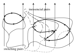
If $A$ is a nonsingular conic with $\mathbb{R}A\neq\varnothing$ and $\mathbb{R}A\subset C$ then the tangency points make a switching pair. The same is true for any convex oval. When an oval is deforming and loses its convexity, new points of tangency may appear. If the deformation is generic, the points of tangency appear and disappear pairwise. Each time appearing pair is an inessential pair of points with distinct indices. Any oval can be deformed (topologically) into a convex one. Tracing the births and deaths of points of tangency it is not difficult to prove the following lemma.
4.2.B [Fie-82, Lemma 2] .
Let $\Gamma$ be a component of $\mathbb{R}A\cap C$ and $M$ be the set of its points of tangency with lines from $Z$. If $\Gamma\cap\partial C=\varnothing$, then $M$ can be divided into pairs, one of which is switching, and all others are inessential. If $\Gamma\cap\partial C\neq\varnothing$, and $\Gamma$ connects distinct boundary lines of $C$ then $M$ can be decomposed into inessential pairs. If the end points of $\Gamma$ are on the same boundary lines of $C$ then $M$ with one point deleted can be decomposed into inessential pairs.$\square$
Denote the closure of $(\mathbb{C}A\smallsetminus\mathbb{R}A)\cap(\bigcup_{t\in I}\mathbb{C}L_{t})$ by $S$. Fix one of the decomposions into pairs of the set of points of tangency of lines from $Z$ with each component of $\mathbb{R}A\cap C$ existing by 4.2.B. By a chain of points of tangency call a sequence of points of tangency, in which any two consecutive points either belong to one of selected pairs or lie in the same component of $S$. A sequence consisting of ovals, on which the selected switching pairs of points of tangency from the chain lie, is called a chain of ovals. Thus the set of ovals of $A$ lying in $C$ appeared to be decomposed to chains of ovals. The next theorem follows obviously from 4.2.A.
4.2.C .
The signs of ovals with respect to $Z$ in a chain alternate (i.e. an oval positive with respect to $Z$ follows by an oval negative with respect to $Z$, the latter oval follows by an oval positive with respect to $Z$). $\square$
The next theorem follows in an obvious way from 4.2.C. Contrary to the previous one, it deals with the signs of ovals with respect to the one-sided component in the case of odd degree and outer ovals in the case of even degree.
4.2.D [Fie-82, Theorem 3].
If the degree of a curve $A$ is odd and ovals of a chain are placed in the same component of the set
| $C\smallsetminus(\text{one-sided component of }\mathbb{R}A)$ |
then the signs of these ovals alternate. If degree of $A$ is even and ovals of a chain are placed in the same component of intersection of $\operatorname{Int}C$ with the interior of the outer oval enveloping these ovals, then the signs of ovals of this chain alternate.$\square$
4.3. Complex Orientations and Pencils of Lines. Alternative Approach
In proofs of 3.8.G, 3.8.H and 3.8.I, the theory developed in the previous section can be replaced by the following Theorem 4.3.A. Although this theorem can be obtained as a corollary of Theorem 4.2.C, it is derived here from Theorem 2.3.A and the complex orientation formula, and in the proof no chain of ovals is used. The idea of this approach to Fiedler’s alternation of orientations is due to V. A. Rokhlin.
4.3.A .
Let $A$ be a non-singular dividing curve of degree $m$. Let $L_{0}$, $L_{1}$ be real lines, $C$ be one of two components of $\mathbb{R}P^{2}\smallsetminus(\mathbb{R}L_{0}\cup\mathbb{R}L_{1})$. Let $\mathbb{R}L_{0}$ and $\mathbb{R}L_{1}$ be oriented so that the projection $\mathbb{R}L_{0}\to\mathbb{R}L_{1}$ from a point lying in $\mathbb{R}P^{2}\smallsetminus(C\cup\mathbb{R}L_{0}\cup\mathbb{R}L_{1})$ preserves the orientations. Let ovals $u_{0}$, $u_{1}$ of $A$ lie in $\mathbb{R}P^{2}-C$ and $u_{i}$ is tangent to $L_{i}$ at one point $(i=1,\,2)$. If the intersection $\mathbb{R}A\cap C$ consists of $m-2$ components, each of which is an arc connecting $\mathbb{R}L_{0}$ with $\mathbb{R}L_{1}$, then points of tangency of $u_{0}$ with $L_{0}$ and $u_{1}$ with $L_{1}$ are positive with respect to one of the complex orientations of $A$.

Proof.
Assume the contrary: suppose that with respect to a complex orientation of $A$ the tangency of $u_{0}$ with $L_{0}$ is positive and the tangency of $u_{1}$ with $L_{1}$ is negative. Rotate $L_{0}$ and $L_{1}$ around the point $L_{0}\cap L_{1}$ in the directions out of $C$ by small angles in such a way that each of the lines $L^{\prime}_{0}$ and $L^{\prime}_{1}$ obtained intersects transversally $\mathbb{R}A$ in $m$ points. Perturb the union $A\cup L^{\prime}_{0}$ and $A\cup L^{\prime}_{1}$ obeying the orientations. By 2.3.A, the nonsingular curves $B_{0}$ and $B_{1}$ obtained are of type I. It is easy to see that their complex schemes can be obtained one from another by relocating the oval, appeared from $u_{1}$ (see Figure 28). This operation changes one of the numbers $\Pi^{+}-\Pi^{-}$ and $\Lambda^{+}-\Lambda^{-}$ by 1. Therefore the left hand side of the complex orientation formula is changed. It means that the complex schemes both of $B_{0}$ and $B_{1}$ can not satisfy the complex orientation formula. This proves that the assumption is not true. $\square$
4.4. Curves of Degree 7
In this section Theorem 3.8.G is proved, i.e. it is proved that there is no nonsingular curve of degree 7 with real scheme $\langle J\amalg\,1\langle 14\rangle\rangle$.
Assume the contrary: suppose that there exists a nonsingular curve $X$ of degree 7 with real scheme $\langle J\amalg\,1\langle 14\rangle\rangle$.
Being an M-curve, $X$ is of type I (see 2.6.B) and, hence, has a complex orientation.
4.4.A Lemma.
$X$ cannot have a complex scheme distinct from $\langle J\amalg\,1^{+}\langle 6^{+}\amalg\,8^{-}\rangle\rangle_{I}^{7}$.
Proof.
Let $\varepsilon$ be the sign of the outer oval, i.e.
| $\varepsilon=\begin{cases}+1,&\text{ if the outer oval is positive}\\ -1,&\text{ otherwise.}\end{cases}$ |
It is clear that
| $\Lambda^{+}=\begin{cases}\Pi^{-}+1,& \text{ if }\varepsilon=+1\\ \Pi^{+},&\text{ if }\varepsilon=-1\end{cases}, \ \ \Lambda^{-}=\begin{cases} \Pi^{+},&\text{ if }\varepsilon=+1\\ \Pi^{-}+1,&\text{ if }\varepsilon=-1. \end{cases}$ |
Therefore, $\Lambda^{+}-\Lambda^{-}=\varepsilon(\Pi^{-}+1-\Pi^{+})$. On the other hand, by 2.7.B, $\Lambda^{+}-\Lambda^{-}=2(\Pi^{-}-\Pi^{+})+3$. From these two equalities we have
| $\varepsilon=2+\frac{1}{\Pi^{-}+1-\Pi^{+}}$ |
and, since $|\varepsilon|=1$, it follows that $\varepsilon=+1$ and $\Pi^{-}+1-\Pi^{+}=-1$, i.e. $\Pi^{+}-\Pi^{-}=2$. Finally, since $\Pi^{+}+\Pi^{-}=14$, it follows that $\Pi^{+}=8$ and $\Pi^{-}=6$. This gives the desired result.$\square$
The next ingredient in the proof of Theorem 3.8.G is a kind of convexity in disposition of interior ovals. Although we study a projective problem, it is possible to speak about convexity, if it is applied to interior ovals. The exact sense of this convexity is provided in the following statement.
4.4.B Lemma.
Let $A$ be any nonsingular curve of degree 7 with real scheme $\langle J\amalg\alpha\amalg 1\langle\beta\rangle\rangle$ and the number of ovals $\geq 6$. Then for each of $\beta$ interior ovals there exists a pair of real lines $L_{1}$, $L_{2}$ intersecting inside this oval such that the rest $\beta-1$ interior ovals lie in one of three domains into which $\mathbb{R}L_{1}\cup\mathbb{R}L_{2}$ cut the disk bounded by the exterior oval.
Proof.
A line intersecting two interior ovals cannot intersect any other interior oval. Furthermore, it intersects each of these two interior ovals in two points, meets the nonempty oval in two points and the one-sided component in one point. (This follows from the following elementary arguments: the line intersects the one-sided component with odd multiplicity, it has to intersect the nonempty oval, since it intersects ovals inside of it, it can intersect any oval with even multiplicty and by Bézout theorem the total number of intersection points is at most 7.) The real point set of the line is divided by the intersection points with the nonempty oval into two segments. One of these segments contains the intersection point with the one-sided component, the other one is inside the nonempty oval and contains the intersections with the interior ovals. A smaller segment connects the interior ovals inside the nonempty ovals. Thus any points inside two interior ovals can be connected by a segment of a line inside the exterior nonemty oval. See Figure 4.4.
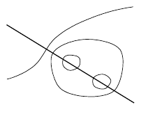
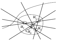
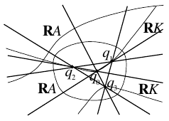
Choose a point inside each interior oval and connect these points by segments inside the exterior oval. If the lines guaranteed by 4.4.B exist, then the segments comprise a convex polygon. Otherwise, there exist interior ovals $u_{0}$, $u_{1}$, $u_{2}$ and $u_{3}$ such that $u_{0}$ is contained inside the triangle made of the segments connecting inside the exterior oval the points $q_{1}$, $q_{2}$, $q_{3}$ chosen inside $u_{1}$, $u_{2}$ and $u_{3}$. See Figure 4.4.
To prove that this is impossible, assume that this is the case and construct a conic $K$ through $q_{1}$, $q_{2}$, $q_{3}$, the point $q_{0}$ chosen inside $u_{0}$ and a point $q_{4}$ chosen inside some empty oval $u_{4}$ distinct from $u_{0}$, $u_{1}$, $u_{2}$ and $u_{3}$ (recall that the total number of ovals is at least 6, thereby $u_{4}$ exists). Since the space of conics is a 5-dimensional real projective space and the conics containing a real point form a real hyperplane, there exists a real conic passing through any 5 real points. If the conic happened to be singular, we could make it nonsingular moving the points. However it cannot happen, since then the conic would be decomposed into two lines and at least one of the lines would intersect with 3 empty ovals and with the nonempty oval, which would contradict the Bézout theorem.
Now let us estimate the number of intersection points of the conic and the original curve $A$ of degree 7. The conic $\mathbb{R}K$ passes through the vertices of the triangle $q_{1}q_{2}q_{3}$ and through the point $q_{0}$ inside it. The component of the intersection of $\mathbb{R}K$ with the interior of the triangle has to be an arc connecting two points of $q_{1}$, $q_{2}$, $q_{3}$. Let they be $q_{1}$ and $q_{2}$. Then the segment $[q_{0},q_{3}]$ lies outside the disk bounded by $\mathbb{R}K$. This segment together with an arc $q_{0},q_{1},q_{3}$ of $\mathbb{R}K$ is a one-sided circle in $\mathbb{R}P^{2}$, which has to intersect the one-sided component of $\mathbb{R}A$. Since neither the segment nor the arc $q_{0},q_{1}$ intersect $\mathbb{R}A$, the arc $q_{1},q_{3}$ does intersect. The intersection point is outside the nonempty oval, while both $q_{1}$ and $q_{3}$ are inside. Therefore the same arc has at least 2 common points with the nonempty oval. Similar arguments show that the arc $q_{2},q_{3}$ intersects the one-sided component of $\mathbb{R}A$ and has at least 2 common points with the nonempty oval. Thus $\mathbb{R}K$ intersects the one-sided component of $A$ at least in 2 points and the nonempty oval at least in 4 points. See Figure 4.4. Together with 10 intersection points with ovals $u_{i}$, $i=0,1,\dots,4$ (2 points with each) it gives 16 points, which contradicts the Bézout theorem. $(^{2})$
$\square$
End of Proof of Theorem 3.8.G.
Assume that a curve $X$ prohibited by Theorem 3.8.G does exist. According to Lemma 4.4.A, its complex scheme is $\langle J\amalg\,1^{+}\langle 6^{+}\amalg\,8^{-}\rangle\rangle_{I}^{7}.$ Take a point inside a positive interior oval. Consider the segment of the pencil of line passing through this point. The other interior ovals compose a chain. By Lemma 4.4.B they lie in one connected component of the intersection of the domain swept by the lines of the segment of the pencil with the interior domain of the nonempty oval. By Theorem 4.2.C signs of ovals in this chain alternate. Therefore the difference between the numbers of positive and negative ovals is 1, while it has to be 3 by Lemma 4.4.A. $\square$
5. Introduction to Topological Study of Real Algebraic Spatial Surfaces
5.1. Basic Definitions and Problems
Our consideration of real algebraic surfaces will be based on definitions similar to the definitions that we used in the case of curves. In particular, by a real algebraic surface of degree $m$ in the 3-dimensional projective space we shall mean a real homogeneous polynomial of degree $m$ in four variables considered up to a constant factor.
Obvious changes adapt definitions of sets of real and complex points, singular points, singular and nonsingular curves and rigid isotopy to the case of surfaces in $\mathbb{R}P^{3}$. Exactly as in the case of curves one formulates the topological classification problem (cf. 1.1.A above):
5.1.A Topological Classification Problem.
Up to homeomorphism, what are the possible sets of real points of a nonsingular real projective algebraic surface of degree $m$ in $\mathbb{R}P^{3}$?
However, the isotopy classification problem 1.1.B splits into two problems:
5.1.B Ambient Topological Classification Problem.
Classify up to homeomorphism the pairs $(\mathbb{R}P^{3},\mathbb{R}A)$ where $A$ is a nonsingular real projective algebraic surface of degree $m$ in $\mathbb{R}P^{3}$?
5.1.C Isotopy Classification Problem.
Up to ambient isotopy, what are the possible sets of real points of a nonsingular a nonsingular real projective algebraic surface of degree $m$ in $\mathbb{R}P^{3}$?
The reason for this splitting is that, contrary to the case of projective plane, there exists a homeomorphism of $\mathbb{R}P^{3}$ non-isotopic to the identity. Indeed, 3-dimensional projective space is orientable, and the mirror reflection of this space in a plane reverses orientation. Thus the reflection is not isotopic to the identity. However, there are only two isotopy classes of homeomorphisms of $\mathbb{R}P^{3}$. It means that the difference between 5.1.B and 5.1.C is not really big. Although the isotopy classification problem is finer, to resolve it, one should add to a solution of the ambient topological classification problem an answer to the following question:
5.1.D Amphichirality Problem.
Which nonsingular real algebraic surfaces of degree $m$ in $\mathbb{R}P^{3}$ are isotopic to its own mirror image?
Each of these problems has been solved only for $m\leq 4$. The difference between 5.1.B and 5.1.C does not appear: the solutions of 5.1.B and 5.1.C coincide with each other for $m\leq 4$. (Thus Problem 5.1.D has a simple answer for $m\leq 4$: any nonsingular real algebraic surface of degree $\leq 4$ is isotopic to its mirror image.) For $m\leq 3$ solutions of 5.1.A and 5.1.B also coincide, but for $m=4$ they are different: there exist nonsingular surfaces of degree 4 in $\mathbb{R}P^{3}$ which are homeomorphic, but embedded in $\mathbb{R}P^{3}$ in a such a way that there is no homeomorphism of $\mathbb{R}P^{3}$ mapping one of them to another. The simplest example is provided by torus defined by equation
| $(x_{1}^{2}+x_{2}^{2}+x_{3}^{2}+3x_{0}^{2})^{2}-16(x_{1}^{2}+x_{2}^{2})x_{0}^{2 }=0$ |
and the union of one-sheeted hyperboloid and an imaginary quadric (perturbed, if you wish to have a surface without singular points even in the complex domain)
Similar splitting happens with the rigid isotopy classification problem. Certainly, it may be transferred literally:
5.1.E Rigid Isotopy Classification Problem.
Classify up to rigid isotopy the nonsingular surfaces of degree $m$.
However, since there exists a projective transformation of $\mathbb{R}P^{3}$, which is not isotopic to the identity (e.g., the mirror reflection in a plane) and a real algebraic surface can be nonisotopic rigidly to its mirror image, one may consider the following rougher problem:
5.1.F Rough Projective Classification Problem.
Classify up to rigid isotopy and projective transformation the nonsingular surfaces of degree $m$.
Again, as in the case of topological isotopy and homeomorphism problem, the difference between these two problems is an amphichirality problem:
5.1.G Rigid Amphichirality Problem.
Which nonsingular real algebraicsurfaces of degree $m$ in $\mathbb{R}P^{3}$ are rigidly isotopic to its mirror image?
Problems 5.1.E, 5.1.F and 5.1.G have been solved also for $m\leq 4$. For $m\leq 3$ the solutions of 5.1.E and 5.1.F coincide with each other and with the solutions of 5.1.A, 5.1.B and 5.1.C. For $m\leq 2$ all these problems belong to the traditional analytic geometry. The solutions are well-known and can be found in traditional textbooks on analytic geometry. The case $m=3$ is also elementary. It was studied in the nineteenth century. The solution is associated with names of Schläfli and Klein. The case $m=4$ is really difficult. Although the first attempts of a serious attack were undertaken in the nineteenth century, too, and among the attackers we see D. Hilbert and K. Rohn, the complete solutions of all classification problems listed above were obtained only in the seventies and eighties. Below, in Subsection LABEL:s5.5n, I will discuss the results and methods. In higher degrees even the most rough problems, like the Harnack problem on the maximal number of components of a surface of degree $m$ are still open.
5.2. Digression: Topology of Closed Two-Dimensional Submanifolds of $\mathbb{R}P^{3}$
For brevity, we shall refer to closed two-dimensional submanifolds of $\mathbb{R}P^{3}$ as topological spatial surfaces, or simply surfaces when there is no danger of confusion.
Since the homology group $H_{2}(\mathbb{R}P^{3};\,\mathbb{Z}_{2})$ is $\mathbb{Z}_{2}$, a connected surface can be situated in $\mathbb{R}P^{3}$ in two ways: zero-homologous, and realizing the nontrivial homology class.
In the first case it divides the projective space into two domains being the boundary for both domains. Hence, the surface divides its tubular neighborhood, i. e. it is two-sided.
In the second case the complement of the surface in the projective space is connected. (If it was not connected, the surface would bound and thereby realize the zero homology class.) Moreover, it is one-sided.
The latter can be proved in many ways. For example, if the surface was two-sided and its complement was connected, there would exist a nontrivial infinite cyclic covering of $\mathbb{R}P^{3}$, which would contradict the fact that $\pi_{1}(\mathbb{R}P^{3})=\mathbb{Z}_{2}.$ The infinite cyclic covering could be constructed by gluing an infinite sequence of copies of $\mathbb{R}P^{3}$ cut along the surface: each copy has to be glued along one of the sides of the cut to the other side of the cut in the next copy.
Another proof: take a projective plane, make it transversal to the surface, and consider the curve which is their intersection. Its homology class in $\mathbb{R}P^{2}$ is the image of the nontrivial element of $H_{2}(\mathbb{R}P^{3};\,\mathbb{Z}_{2})$ under the inverse Hopf homomorphism $in^{!}:H_{2}(\mathbb{R}P^{3};\,\mathbb{Z}_{2})\to H_{1}(\mathbb{R}P^{2};\, \mathbb{Z}_{2})$. This is an isomorphism, as one can see taking the same construction in the case when the surface is another projective plane. Thus the intersection is a one-sided curve in $\mathbb{R}P^{2}$. Hence the normal fibration of the original surface in $\mathbb{R}P^{3}$ is not trivial. This means that the surface is one-sided.
A connected surface two-sidedly embedded in $\mathbb{R}P^{3}$ is orientable, since it bounds a part of the ambient space which is orientable. Therefore, such a surface is homeomorphic to sphere or to sphere with handles. There is no restriction to the number of handles: one can take an embedded sphere bounding a small ball, and adjoin to it any number of handles.
A one-sidedly embedded surface is nonorientable. Indeed, its normal bundle is nonorientable, while the restriction of the tangent bundle of $\mathbb{R}P^{3}$ to the surface is orientable (since $\mathbb{R}P^{3}$ is). The restriction of the tangent bundle of $\mathbb{R}P^{3}$ to the surface is the Whitney sum of the normal and tangent bundles of the surface. Therefore it cannot happen that only one of these three bundles is not orientable.
Contrary to the case of two-sided surfaces, in the case of one-sided surfaces there is an additional restriction on their topological types.
5.2.A .
The Euler characteristic of a connected surface one-sidedly embedded to $\mathbb{R}P^{3}$ is odd.
In particular, it is impossible to embed a Klein bottle to $\mathbb{R}P^{3}$. (The Euler characteristic of a connected surface two-sidedly embedded into $\mathbb{R}P^{3}$ is even, but it follows from orientability: the Euler characteristic of any closed oriented surface is even.) By topological classification of closed surfaces, a nonorientable connected surface with odd Euler characteristic is homeomorphic to the projective plane or to the projective plane with handles. Any surface of this sort can be embedded into $\mathbb{R}P^{3}$: for the projective plane $\mathbb{R}P^{3}$ is the native ambient space, and one can adjoin to it in $\mathbb{R}P^{3}$ any number of handles. We denote a sphere with $g$ handles by $S_{g}$ and a projective plane with $g$ handles by $P_{g}$.
Proof of 5.2.A.
Let $S$ be a connected surface one-sidedly embedded into $\mathbb{R}P^{3}$. By a small shift it can be made transversal to the projective plane $\mathbb{R}P^{2}$ standardly embedded into $\mathbb{R}P^{3}$. Since both surfaces are embedded one-sidedly, they realize the same homology class in $\mathbb{R}P^{3}$. Therefore their union bounds in $\mathbb{R}P^{3}$: one can color the complement $\mathbb{R}P^{3}\smallsetminus(S\cup\mathbb{R}P^{2})$ into two colors in such a way that the components adjacent from the different sides to the same (two-dimensional) piece of $S\cup\mathbb{R}P^{2}$ would be of different colors. It is a kind of checkerboard coloring.
Consider the disjoint sum $Q$ of the closures of those components of $\mathbb{R}P^{3}\smallsetminus(S\cup\mathbb{R}P^{2})$ which are colored with the same color. It is a compact 3-manifold. It is oriented since each of the components inherits orientation from $\mathbb{R}P^{3}$. The boundary of this 3-manifold is composed of pieces of $S$ and $\mathbb{R}P^{2}$. It can be thought of as the result of cutting both surfaces along their intersection curve and regluing. The intersection curve is replaced by its two copies, while the rest part of $S$ and $\mathbb{R}P^{2}$ does not change. Since the intersection curve consists of circles, its Euler characteristic is zero. Therefore $\chi(\partial Q)=\chi(S)+\chi(\mathbb{R}P^{2})=\chi(S)+1$. On the other hand, $\chi(\partial Q)$ is even since $\partial Q$ is a closed oriented surface ($\partial Q$ inherits orientation from $Q$). Thus $\chi(S)$ is odd. $\square$
A one-sided connected surface in $\mathbb{R}P^{3}$ contains a loop which is not contractible in $\mathbb{R}P^{3}$. Such a loop can be detected in the following way: Consider the intersection of the surface with any one-sided transversal surface (e. g., $\mathbb{R}P^{2}$ or a surface obtained from the original one by a small shift). The homology class of the intersection curve is the self-intersection of the nonzero element of $H_{2}(\mathbb{R}P^{3}\,;\,\mathbb{Z}_{2})$. Since the self-intersection is the nonzero element of $H_{1}(\mathbb{R}P^{3}\,;\,\mathbb{Z}_{2})$, the intersection curve contains a component noncontractible in $\mathbb{R}P^{3}$.
A two-sided connected surface in $\mathbb{R}P^{3}$ can contain no loops noncontractible in $\mathbb{R}P^{3}$ (this happens, for instance, if the surface lies in an affine part of $\mathbb{R}P^{3}$). Of course, if a surface contains a loop noncontractible in $\mathbb{R}P^{3}$, it is not contractible in $\mathbb{R}P^{3}$ itself. Moreover, then it meets any one-sided surface, since the noncontractible loop realizes the nonzero element of $H_{1}(\mathbb{R}P^{3}\,;\,\mathbb{Z}_{2})$ and this element has nonzero intersection number with the homology class realized by a one-sided surface.
If any loop on a connected surface $S$ embedded in $\mathbb{R}P^{3}$ is contractible in $\mathbb{R}P^{3}$ (which means that the embedding homomorphism $\pi_{1}(S)\to\pi_{1}(\mathbb{R}P^{3})$ is trivial), then there is no obstruction to contract the embedding, i. e., to construct a homotopy between the embedding $S\to\mathbb{R}P^{3}$ and a constant map. One can take a cell decomposition of $S$, contract the 1-skeleton (extending the homotopy to the whole $S$), and then contract the map of the 2-cell, which is possible, since $\pi_{2}(\mathbb{R}P^{3})=0$. A surface of this sort is called contractible (in $\mathbb{R}P^{3}$).
It may happen, however, that there is no isotopy relating the embedding of a contractible surface with a map to an affine part of $\mathbb{R}P^{3}$. The simplest example of a contractible torus which cannot be moved by an isotopy to an affine part of $\mathbb{R}P^{3}$ is shown in Figure 32.

As it was stated above, the complement $\mathbb{R}P^{3}\smallsetminus S$ of a connected surface $S$ two-sidedly embedded in $\mathbb{R}P^{3}$ consists of two connected components. If $S$ is not contractible in $\mathbb{R}P^{3}$ then both of them are not contractible, since a loop on $S$ noncontractible in $\mathbb{R}P^{3}$ can be pushed to each of the components. They may be positioned in $\mathbb{R}P^{3}$ in the same way.
The simplest example of this situation is provided by a one-sheeted hyperboloid. It is homeomorphic to torus and its complement consists of two solid tori. So, this is a Heegaard decomposition of $\mathbb{R}P^{3}$. There exists an isotopy of $\mathbb{R}P^{3}$ made of projective transformation exchanging the components. $(^{3})$
A connected surface decomposing $\mathbb{R}P^{3}$ into two handlebodies is called a Heegaard surface. Heegaard surfaces are the most unknotted surfaces among two-sided noncontractible connected surfaces. They may be thought of as unknotted noncontractible surfaces.
If a connected surface $S$ is contractible in $\mathbb{R}P^{3}$, then the components $C_{1}$ and $C_{2}$ can be distinguished in the following way: for one of them, say $C_{1}$, the inclusion homomorphism $\pi_{1}(C_{1})\to\pi_{1}(\mathbb{R}P^{3})$ is trivial, while for the other one the inclusion homomorphism $\pi_{1}(C_{2})\to\pi_{1}(\mathbb{R}P^{3})$ is surjective. This follows from the van Kampen theorem. The component with trivial homomorphism is called the interior of the surface. It is contractible in $\mathbb{R}P^{3}$ (in the same sense as the surface is).
A contractible connected surface $S$ in $\mathbb{R}P^{3}$ is said to be unknotted, if it is contained in some ball $B$ embedded into $\mathbb{R}P^{3}$ and divides this ball into a ball with handles (which is the interior of $S$) and a ball with handles with an open ball deleted. Any two unknotted contractible surfaces of the same genus are ambiently isotopic in $\mathbb{R}P^{3}$. Indeed, first the balls containing them can be identified by an ambient isotopy (see, e. g., Hirsch Hir-76, Section 8.3), then it follows from uniqueness of Heegaard decomposition of sphere that there is an orientation preserving homeomorphism of the ball mapping one of the surfaces to the other. Any orientation preserving homeomorphism of a 3-ball is isotopic to the identity.
At most one component of a (closed) surface embedded in $\mathbb{R}P^{3}$ may be one-sided. Indeed, a one-sided closed surface cannot be zero-homologous in $\mathbb{R}P^{3}$ and the self-intersection of its homology class (which is the only nontrivial element of $H_{2}(\mathbb{R}P^{3}\,;\,\mathbb{Z}_{2})$) is the nonzero element of $H_{1}(\mathbb{R}P^{3}\,;\,\mathbb{Z}_{2})$. Therefore any two one-sided surfaces in $\mathbb{R}P^{3}$ intersect.
Moreover, if an embedded surface has a one-sided component, then all other components are contractible. The contractible components are naturally ordered: a contractible component of a surface can contain other contractible component in its interior and this gives rise to a partial order in the set of contractible components. If the interior of contractible surface $A$ contains a surface $B$, then one says that $A$ envelopes $B$.
The connected components of a surface embedded in $\mathbb{R}P^{3}$ divide $\mathbb{R}P^{3}$ into connected regions. Let us construct a graph of adjacency of these regions: assign a vertex to each of the regions and connect two regions with an edge if the corresponding regions are adjacent to the same connected two-sided component of the surface. Since the projective space is connected and its fundamental group is finite, the graph is contractible, i. e., it is a tree. It is called region tree of the surface.
Consider now a (closed) surface without one-sided components. It may contain several noncontractible components. They decompose the projective space into connected domains, each of which is not contractible in $\mathbb{R}P^{3}$. Let us construct a graph of adjacency of these domains: assign a vertex to each of the domains and connect two vertices with an edge if the corresponding domains are adjacent. Edges of the graph correspond to noncontractible components of the surface. For the same reasons as above, this graph is contractible, i. e. it is a tree. This tree is called the domain tree of the surface.
Contractible components of the surface are distributed in the domains. Contractible components which are contained in different domains cannot envelope one another. Contractible components of the surface which lie in the same domain are partially ordered by enveloping. They divide the domain into regions. Each domain contains only one region which is not contractible in $\mathbb{R}P^{3}$. If the domain does not coincide with the whole $\mathbb{R}P^{3}$ (i.e., the surface does contain noncontractible components), then this region can be characterized also as the only region which is adjacent to all the noncontractible components of the surface comprising the boundary of the domain. Indeed, contractible components of the surface cannot separate noncontractible ones.
The region tree of a surface contains a subtree isomorphic to the domain tree, since one can assign to each domain the unique noncontractible region contained in the domain and two domains are adjacent iff the noncontractible regions contained in them are adjacent. The complement of the noncontractible domains tree is a union of adjacency trees for contractible subdomains contained in each of the domains.
Let us summarize what can be said about topology of a spatial surface in the terms described above.
If a surface is one-sided (i. e., contains a one-sided component), then it is a disjoint sum of a projective plane with handles and several (maybe none) spheres with handles. Thus, it is homeomorphic to
| $P_{g}\amalg S_{g_{1}}\amalg\dots S_{g_{k}},$ |
where $\amalg$ denotes disjoint sum.
All two-sided components are contractible and ordered by enveloping. The order is easy to incorporate into the notation of the topological type above. Namely, place notations for components enveloped by a component $A$ immediately after $A$ inside brackets $\langle\ \rangle$. For example,
| $P_{0}\amalg S_{1}\amalg S_{1}\amalg S_{0}\langle S_{1}\amalg S_{0}\amalg S_{2} \langle S_{1}\amalg S_{0}\rangle\amalg S_{2}\langle S_{1}\amalg S_{0}\rangle\rangle$ |
denotes a surface consisting of a projective plane, two tori, which do not envelope any other component, a sphere, which envelopes a torus and a sphere without components inside them and a two spheres with two handles each of which envelopes empty sphere and torus. To make the notations shorter, let us agree to skip index 0, i. e. denote projective plane $P_{0}$ by $P$ and sphere $S_{0}$ by $S$, and denote the disjoint sum of $k$ fragments identical to each other by $k$ followed by the notation of the fragment. These agreements shorten the notation above to
| $P\amalg 2S_{1}\amalg S\langle S_{1}\amalg S\amalg 2S_{2}\langle S_{1}\amalg S \rangle\rangle.$ |
If a surface is two-sided (i. e. does not contain a one-sided component), then it is a disjoint sum $S_{g_{1}}\amalg\dots S_{g_{k}},$ of spheres with handles. To distinguish in notations the components noncontractible in $\mathbb{R}P^{3}$, we equip the corresponding symbols with upper index 1. Although we do not make any difference between two components of the complement of noncontractible connected surface (and there are cases when they cannot be distinguished), in notations we proceed as if one of the components is interior: the symbols denoting components of the surface which lie in one of the components of the complement of the noncontractible component $A$ are placed immediately after the notation of $A$ inside braces $\{\ \}$. Our choice is the matter of convenience. It correspond to the well-known fact that usually, to describe a tree, one introduces a partial order on the set of its vertices.
In these notations,
| $S_{1}\amalg S\langle 3S\rangle\amalg S_{1}^{1}\{S_{3}\amalg 2S_{2}^{1}\{3S \amalg S_{1}\}\}$ |
denotes a two-sided surface containing three noncontractible components. One of them is a torus, two others are spheres with two handles. The torus bounds a domain containing a contractible empty torus and a sphere enveloping three empty spheres. There is a domain bounded by all three noncontractible components. It contains a contractible empty sphere with three handles. Each of the noncontractible spheres with two handles bounds a domain containing empty contractible torus and three empty spheres.
This notation system is similar to notations used above to described isotopy types of curves in the projective plane. However, there is a fundamental difference: the notations for curves describe the isotopy type of a curve completely, while the notations for surfaces are far from being complete in this sense. Although topological type of the surface is described, knotting and linking of handles are completely ignored. In the case when there is no handle, the notation above does provide a complete description of isotopy type.
5.3. Restrictions on Topology of Real Algebraic Surfaces
As in the case of real plane projective curves, the set of real points of a nonsingular spatial surface of degree $m$ is one-sided, if $m$ is odd, and two-sided, if $m$ is even. Indeed, by the Bézout theorem a generic line meets a surface of degree $m$ in a number of points congruent to $m$ modulo 2. On the other hand, whether a topological surface embedded in $\mathbb{R}P^{3}$ is one-sided or two-sided, can be detected by its intersection number modulo 2 with a generic line: a surface is one-sided, iff its intersection number with a generic line is odd.
There are some other restrictions on topology of a nonsingular surface of degree $m$ which can be deduced from the Bézout theorem.
5.3.A On Number of Cubic’s Components.
The set of real points of a nonsingular surface of degree three consists of at most two components.
Proof.
Assume that there are at least three components. Only one of them is one-sided, the other two are contractible. Connect with a line two contractible components. Since they are zero-homologous, the line should intersect each of them with even intersection number. Therefore the total number of intersection points (counted with multiplicities) of the line and the surface is at least four. This contradicts to the Bézout theorem, according to which it should be at most three.$\square$
5.3.B On Two-Component Cubics.
If the set of real points of a nonsingular surface of degree 3 consists of two components, then the components are homeomorphic to the sphere and projective plane (i. e., this is $P\amalg S$).
Proof.
Choose a point inside the contractible component. Any line passing through this point intersects the contractible component at least in two points. These points are geometrically distinct, since the line should intersect also the one-sided component. On the other hand, the total number of intersection points is at most three according to the Bézout theorem. Therefore any line passing through the selected point intersects one-sided component exactly in one point and two-sided component exactly in two points. The set of all real lines passing through the point is $\mathbb{R}P^{2}$. Drawing a line through the selected point and a real point of the surface defines a one-to-one map of the one-sided component onto $\mathbb{R}P^{2}$ and two-to-one map of the two-sided component onto $\mathbb{R}P^{2}$. Therefore the Euler characteristic of the one-sided component is equal to $\chi(\mathbb{R}P^{2})=1$, and the Euler characteristic of the two-sided component is $2\chi(\mathbb{R}P^{2})=2$. This determines the topological types of the components. $\square$
5.3.C Estimate for Diameter of Region Tree.
The diameter of the region tree66Here by the diameter of a tree it is understood the maximal number of edges in a simple chain of edges of the tree, i. e., the diameter of the tree in the internal metric, with respect to which each edge has length 1. of a nonsingular surface of degree $m$ is at most $[m/2]$.
Proof.
Choose two vertices of the region tree the most distant from each other. Choose a point in each of the coresponding regions and connect the points by a line. $\square$
5.3.D .
The set of real points of a nonsingular surface of degree 4 has at most two noncontractible components. If the number of noncontractible components is 2, then there is no other component.
Proof.
First, assume that there are at least three noncontractible components. Consider the complement of the union of three noncontractible components. It consists of three domains, and at least two of them are not adjacent (cf. the previous subsection: the graph of adjacency of the domains should be a tree). Connect points of nonadjacent domains with a line. It has to intersect each of the three noncontractible components. Since they are zero-homologous, it intersects each of them at least in two points. Thus, the total number intersection points is at least 6, which contradicts to the Bézout theorem.
Now assume that there are two noncontractible components and some contractible component. Choose a point $p$ inside the contractible component. The noncontractible components divide $\mathbb{R}P^{3}$ into 3 domains. One of the domains is adjacent to the both noncontractible components, while each of the other two domains is bounded by a single noncontractible component. If the contractible component lies in a domain bounded by a single noncontractible component, then take a point $q$ in the other domain of the same sort, and connect $p$ and $q$ with a line. This line meets each of the three components at least twice, which contradicts to the Bézout theorem.
Otherwise (i. e. if the contractible component lies in the domain adjacent to both noncontractible components), choose inside each of the two other domains an embedded circle, which does not bound in $\mathbb{R}P^{3}$. Denote these circles by $L_{1}$ and $L_{2}$. Consider a surface $C_{i}$ swept by lines connecting $p$ with points of $L_{i}$. It realizes the nontrivial homology class. Indeed, take any line $L$ transversal to it. Each point of $L\cap C_{i}$ corresponds to a point of the intersection of $L_{i}$ and the plane consisting of lines joining $p$ with $L$. Since $L_{i}$ realizes the nonzero homology class, the intersection number of $L_{i}$ with a plane is odd. Therefore the intersection number of $L$ and $C_{i}$ is odd. Since both $C_{1}$ and $C_{2}$ realizes the nontrivial homology class, their intersection realizes the nontrivial one-dimensional homology class. This may happen only if there is a line passing through $p$ and meeting $L_{1}$ and $L_{2}$. Such a line has to intersect all three components of the quadric surface. Each of the components has to be met at least twice. This contradicts to the Bézout theorem.$\square$
5.3.E Remark.
In fact, if a nonsingular quartic surface has two noncontractible components then each of them is homeomorphic to torus. It follows from an extremal property of the refined Arnold inequality 5.3.L. I do not know, if it can be deduced from the Bézout theorem. However, if to assume that one can draw lines in the domains of the complement which are not adjacent to both components, then it is not difficult to find homeomorphisms between the components of the surface and the torus, which is the product of these two lines. Cf. the proof of 5.3.B.
5.3.F Generalization of 5.3.D.
Let $A$ be a nonsingular real algebraic surface of degree $m$ in the 3-dimensional projective space. Then the diameter of the adjacency tree of domains of the complement of $\mathbb{R}A$ is at most $[m/2]$. If the degree is even and the diameter of the adjacency tree of the connected components of the complement of the union of the noncontractible components is exactly $m/2$, then there is no contractible components.
The proof is a straightforward generalization of the proof of 5.3.D.$\square$
Surprisingly, Bézout theorem gave much less restrictions in the case of surfaces than in the case of plane curves. In particular, it does not give anything like Harnack Inequality. Most of restrictions on topology of surfaces are analogous to the restrictions on flexible curves and were obtained using the same topological tools. Here is a list of the restrictions, though it is non-complete in any sense.
The restrictions are formulated below for a nonsingular real algebraic surface $A$ of degree $m$ in the 3-dimensional projective space. In these formulations and in what follows we shall denote the $i$-th Betti number of $X$ over field $\mathbb{Z}_{2}$ (which is nothing but $\dim_{\mathbb{Z}_{2}}H_{i}(X\,;\,\mathbb{Z}_{2})$) by $b_{i}(X)$. In particular, $b_{0}(X)$ is the number of components of $X$. By $b_{*}(X)$ we denote the total Betti number, i. e. $\sum_{i=0}^{infty}b_{i}(X)=\dim_{\mathbb{Z}_{2}}H_{*}(X\,;\,\mathbb{Z}_{2})$.
5.3.G Generalized Harnack Inequality.
| $b_{*}(\mathbb{R}A)\leq m^{3}-4m^{2}+6m.$ |
5.3.H Remark.
This is a special case of Smith-Floyd Theorem 3.2.B, which in the case of curves implies Harnack Inequality, see Subsections 3.2. It says that for any involution $i$ of a topological space $X$
| $b_{*}(fix(i))\leq b_{*}(X).$ |
Applying this to the complex conjugation involution of the complexification $\mathbb{C}A$ of $A$ and taking into account that $\dim_{\mathbb{Z}_{2}}H_{*}(\mathbb{C}A\,;\,\mathbb{Z}_{2})=m^{3}-4m^{2}+6m$ one gets 5.3.G. Applications to high-dimensional situation is discussed in Subsection LABEL:s15.1d below.
5.3.I Extremal Congruences of Generalized Harnack Inequality.
If
| $b_{*}(\mathbb{R}A)=m^{3}-4m^{2}+6m,$ |
then
| $\chi(\mathbb{R}A)\equiv(4m-3m^{2})/3\mod 16.$ |
If $b_{*}(\mathbb{R}A)=m^{3}-4m^{2}+6m-2$, then
| $\chi(\mathbb{R}A)\equiv(4m-m^{3}\pm 6)/3\mod 16.$ |
5.3.J Petrovsky - Oleinik Inequalities.
| $-(2m^{3}-6m^{2}+7m-6)/3\leq\chi(\mathbb{R}A)\leq(2m^{3}-6m^{2}+7m)/3.$ |
Denote the numbers of orientable components of $\mathbb{R}A$ with positive, zero and negative Euler characteristic by $k^{+}$, $k^{0}$ and $k^{-}$ respectively.
5.3.K Refined Petrovsky - Oleinik Inequality.
If $m\not=2$ then
| $-(2m^{3}-6m^{2}+7m-6)/3\leq\chi(\mathbb{R}A)-2k^{+}-2k^{0}.$ |
5.3.L Refined Arnold Inequality.
Either $m$ is even, $k^{+}=k^{-}=0$ and
| $k^{0}=(m^{3}-6m^{2}+11m)/6,$ |
or
| $k^{0}+k^{-}\leq(m^{3}-6m^{2}+11m-6)/6.$ |
5.4. Surfaces of Low Degree
Surfaces of degree 1 and 2 are well-known. Any surface of degree 1 is a projective plane. All of them are transformed to each other by a rigid isotopy consisting of projective transformations of the whole ambient space $\mathbb{R}P^{3}$.
Nonsingular surfaces of degree 2 (nonsingular quadrics) are of three types. It follows from the well-known classification of real nondegenerate quadratic forms in 4 variables up to linear transformation. Indeed, by this classification any such a form can be turned to one of the following:
-
(1)
$+x_{0}^{2}+x_{1}^{2}+x_{2}^{2}+x_{3}^{2}$,
-
(2)
$+x_{0}^{2}+x_{1}^{2}+x_{2}^{2}-x_{3}^{2}$,
-
(3)
$+x_{0}^{2}+x_{1}^{2}-x_{2}^{2}-x_{3}^{2}$,
-
(4)
$+x_{0}^{2}-x_{1}^{2}-x_{2}^{2}-x_{3}^{2}$,
-
(5)
$-x_{0}^{2}-x_{1}^{2}-x_{2}^{2}-x_{3}^{2}$.
Multiplication by $-1$ identifies the first of them with the last and the second with the fourth reducing the number of classes to three. Since the reduction of a quadratic form to a canonical one can be done in a continuous way, all quadrics belonging to the same type also can be transformed to each other by a rigid isotopy made of projective transformations.
The first of the types consists of quadrics with empty set of real points. In traditional analytic geometry these quadrics are called imaginary ellipsoids. A canonical representative of this class is defined by equation $x_{0}^{2}+x_{1}^{2}+x_{3}^{2}+x_{4}^{2}=0$.
The second type consists of quadrics with the set of real points homeomorphic to sphere. In the notations of the previous section this is $S$. The canonical equation is $x_{0}^{2}+x_{1}^{2}+x_{2}^{2}-x_{3}^{2}=0$.
The third type consists of quadrics with the set of real points homeomorphic to torus. They are known as one-sheeted hyperboloids. The set of real points is not contractible (it contains a line), so in the notations above it should be presented as $S_{1}^{1}$. The canonical equation is $x_{0}^{2}+x_{1}^{2}-x_{2}^{2}-x_{3}^{2}=0$.
Quadrics of the last two types (i. e., quadrics with nonempty real part) can be obtained by small perturbations of a union of two real planes. To obtain a quadric with real part homeomorphic to sphere, one may perturb the union of two real planes in the following way. Let the plane be defined by equations $L_{1}(x_{0},x_{1},x_{2},x_{3})=0$ and $L_{2}(x_{0},x_{1},x_{2},x_{3})=0$. Then the union is defined by equation $L_{1}(x_{0},x_{1},x_{2},x_{3})L_{2}(x_{0},x_{1},x_{2},x_{3})=0$. Perturb this equation adding a small positive definite quadratic form. Say, take
| $L_{1}(x_{0},x_{1},x_{2},x_{3})L_{2}(x_{0},x_{1},x_{2},x_{3})+\varepsilon(x_{0} ^{2}+x_{1}^{2}+x_{2}^{2}+x_{3}^{2})=0$ |
with a small $\varepsilon>0$. This equation defines a quadric. Its real part does not meet plane $L_{1}(x_{0},x_{1},x_{2},x_{3})=L_{2}(x_{0},x_{1},x_{2},x_{3})$, since on the real part of the quadric the product $L_{1}(x_{0},x_{1},x_{2},x_{3})L_{2}(x_{0},x_{1},x_{2},x_{3})$ is negative. Therefore the real part of the quadric is contractible in $\mathbb{R}P^{3}$. Since it is obtained by a perturbation of the union of two planes, it is not empty, provided $\varepsilon>0$ is small enough. As easy to see, it is not singular for small $\varepsilon>0$. Cf. Subsection LABEL:s11.5d. Of course, this can be proved explicitely, as an exercise in analytic geometry. See Figure 33
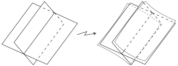
To obtain a noncontractible nonsingular quadric (one-sheeted hyperboloid), one can perturb the same equation $L_{1}(x_{0},x_{1},x_{2},x_{3})L_{2}(x_{0},x_{1},x_{2},x_{3})=0$, but by a small form which takes both positive and negative values on the intersection line of the planes. See Figure 34.
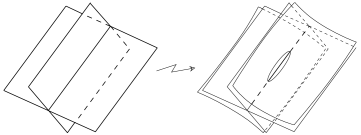
Nonsingular surfaces of degree 3 (nonsingular cubics) are of five types. Here is the complete list of there topological types:
| $P,\quad P\amalg S,\quad P_{1},\quad P_{2},\quad P_{3}.$ |
Let us prove, first, that only topological types from this list can be realized. Since the degree is odd, a nonsingular surface has to be one-sided. By 5.3.D if it is not connected, then it is homeomorphic to $P\amalg S$. By the Generalized Harnack Inequality 5.3.G, the total Betti number of the real part is at most $3^{3}-4\times 3^{2}+6\times 3=9$. On the other hand, the first Betti number of a projective plane with $g$ handles is $1+2g$ and the total Betti number $b_{*}(P_{g})$ is $3+2g$. Therefore in the case of a nonsingular cubic with connected real part, it is of the type $P_{g}$ with $g\leq 3$.
All the five topological types are realized by small perturbations of unions of a nonsingular quadric and a plane transversal to one another. This is similar to the perturbations considered above, in the case of spatial quadrics. See Figures 35 and 36.
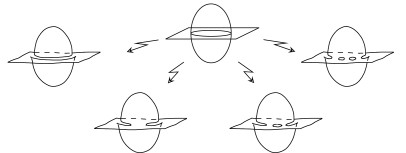
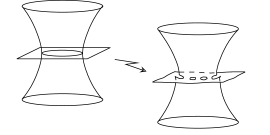
An alternative way to construct nonsingular surfaces of degree 3 of all the topological types is provided by a connection between nonsingular spatial cubics and plane nonsingular quartics. More precisely, there is a correspondence assigning a plane nonsingular quartic with a selected real double tangent line to a nonsingular spatial cubic with a selected real point on it. It goes as follows. Consider the projection of the cubic from a point selected on it to a plane. The projection is similar to the well-known stereographic projection of a sphere to plane.
References
- A’C-79 N. A’Campo, Sur la première partie du 16e problème de Hilbert, Sem. Bourbaki 537 (1979).
- Arn-71 V. I. Arnold, On the location of ovals of real algebraic plane curves, involutions on four-dimensional smooth manifolds, and the arithmetic of integral quadratic forms, Funktsional. Anal. i Prilozhen 5 (1971), 1–9.
- Arn-73 V. I. Arnold, Topology of real algebraic curves (I. G. Petrovsky’s works and their development), Uspekhi Mat. Nauk 28 (1973), 260–262 (Russian).
- Arn-79 V. I. Arnold and O. A. Oleĭnik, The topology of real algebraic manifolds, Vestnik Moscov. Univ. 1 (1979), 7–17.
- AVGZ-82 V. I. Arnold, A. N. Varchenko, and S. M. Gusein-Zade, Singularities of differentiable maps. I, “Nauka”, Moscow, 1982 (Russian), English transl., Birkhaüser, Basel, 1985.
- Bre-72 G. Bredon, Introduction into compact transformation groups, Academic Press, New York, London, 1972.
- Bru-56 L. Brusotti, Su talune questioni di realita nei loro metodi, resultati e pro le me, Collogue sur les Questions de Réalite en Geometrie., Georges Johne, Liege, and Masson, Paris, 1956, Liege, 1955, pp. 105–129 (Italian).
- Dan-78 V. I. Danilov, The geometry of toric manifolds, Uspekhi Mat. Nauk 33 (1978), 85–134 (Russian), English transl., Russian Math. Surveys 33:2 (1978).
- Fie-82 T. Fiedler, Pencils of lines and topology of real algebraic curves, Izv. Akad. Nauk, Ser. Mat. 46 (1982), 853–863 (Russian), MR 84e:14019. Math. USSR-Izv.21(1983), 161–170.
- Fie-83 T. Fiedler, New congruences in the topology of real plane algebraic curves, Dokl. Akad. Nauk SSSR 270 (1983).
- GK-73 D. A. Gudkov and A. D. Krakhnov, On the periodicity of the Euler characteristic of real algebraic ${M}-1$-manifolds, Funktsional Anal. i Prilozhen. 7 (1973), 15–19 (Russian).
- GM-77 L. Guillou and A. Marin, Une extension d’un théorem de Rohlin sur la signature, C. R. Acad. Sci. Paris 285 (1977), 95–97.
- GU-69 D. A. Gudkov and G. A. Utkin, The topology of curves of degree 6 and surfaces of degree 4, Uchen. Zap. Gorkov. Univ., vol. 87, 1969 (Russian), English transl., Transl. AMS 112.
- Gud-71 D. A. Gudkov, Construction of a new series of ${M}$-curves, Dokl. Akad. Nauk SSSR 200 (1971), 1269–1272 (Russian).
- Gud-73 D. A. Gudkov, Construction of a curve of degree 6 of type $\tfrac{5}{1}5$, Izv. Vyssh. Uchebn. Zaved. Mat. 3 (1973), 28–36 (Russian).
- Gud-74 D. A. Gudkov, The topology of real projective algebraic varieties, Uspekhi Mat. Nauk 29 (1974), 3–79 (Russian), English transl., Russian Math. Surveys 29:4 (1974), 1–79.
- Har-76 A. Harnack, Über Vieltheiligkeit der ebenen algebraischen Curven, Math. Ann. 10 (1876), 189–199.
- Hil-91 D. Hilbert, Über die reellen Züge algebraischen Curven, Math. Ann. 38 (1891), 115–138.
- Hil-01 D. Hilbert, Mathematische Probleme, Arch. Math. Phys. 3 (1901), 213–237 (German).
- Hir-76 M. W. Hirsch, Differential topology, Springer-Verlag, New York, Heidelberg, Berlin, 1976.
- Ite-93 I. V. Itenberg, Countre-ememples à la conjecture de Ragsdale, C. R. Acad. Sci. Paris 317 (1993), 277–282.
- Kha-73 V. M. Kharlamov, New congruences for the Euler characteristic of real algebraic varieties, Funksional. Anal. i Prilozhen. 7 (1973), 74–78 (Russian).
- Kha-78 V. M. Kharlamov, Real algebraic surfaces, Proc. Internat. Congr. Math., Helsinki (1978), 421–428.
- Kha-86 V. M. Kharlamov, The topology of real algebraic manifolds (commentary on papers N${}^{\circ}$ 7,8), I. G. Petrovskiĭ’s Selected Works, Systems of Partial Differential Equations, Algebraic Geometry,, Nauka, Moscow, 1986, pp. 465–493 (Russian).
- Kle-22 F. Klein, Gesammelte mathematische Abhandlungen, vol. 2, Berlin, 1922.
- KV-88 V. M. Kharlamov and O. Ya. Viro, Extensions of the Gudkov-Rokhlin congruence, Lecture Notes in Math., vol. 1346, Springer, 1988, pp. 357–406.
- Mar-80 A. Marin, Quelques remarques sur les courbes algebriques planes reelles, Publ. Math. Univ. Paris VII 9 (1980).
- Mik-94 G. B. Mikhalkin, The complex separation of real surfaces and extensions of Rokhlin congruence, Invent. Math. 118 (1994), 197–222.
- Mil-69 J. Milnor, Morse theory, Princeton Univ. Press, Princeton, N.J., 1969.
- Mis-75 N. M. Mishachev, Complex orientations of plane ${M}$-curves of odd degree, Funktsional Anal. i Prilozhen. 9 (1975), 77–78 (Russian).
- Ole-51 O. A. Oleĭnik, On the topology of real algebraic curves on an algebraic surface, Mat. Sb. 29 (1951), 133–156 (Russian).
- Nik-83 V. V. Nikulin, Involutions of integer quadratic forms and their applications to real algebraic geometry, Izv. Akad. Nauk SSSR Ser. Mat. 47 (1983).
- Pet-33 I. Petrovski, Sur le topologie des courbes réelles et algèbriques, C. R. Acad. Sci. Paris (1933), 1270–1272.
- Pet-38 I. Petrovski, On the topology of real plane algebraic curves, Ann. of Math. 39 (1938), 187–209.
- PO-49 I. G. Petrovskiĭ and O. A. Oleĭnik, On the topology of real algebraic surfaces, Izv. Akad. Nauk SSSR Ser. Mat. 13 (1949), 389–402 (Russian).
- Rag-06 V. Ragsdale, On the arrangement of the real branches of plane algebraic curves, Amer. J. Math. 28 (1906), 377–404.
- Roh-13 K. Rohn, Die Maximalzahl und Anordnung der Ovale bei der ebenen Curve 6. Ordnung und bei Flache 4. Ordnung, Math. Ann. 73 (1913), 177–229.
- Rok-72 V. A. Rokhlin, Congruences modulo 16 in Hilbert’s sixteenth problem, Funktsional. Anal. i Prilozhen. 6 (1972), 58–64 (Russian).
- Rok-74 V. A. Rokhlin, Complex orientations of real algebraic curves, Funktsional. Anal. i Prilozhen. 8 (1974), 71–75 (Russian).
- Rok-78 V. A. Rokhlin, Complex topological characteristics of real algebraic curves, Uspekhi Mat. Nauk 33 (1978), 77–89 (Russian).
- Rok-80 V. A. Rokhlin, New inequalities in the topology of real plane algebraic curves, Funktsional. Anal. i Prilozhen. 14 (1980), 37–43 (Russian), MR 82a:14066. Functional Anal. Appl. 14(1980), 29–33.
- Sha-77 I. R. Shafarevich, Basic algebraic geometry, Springer-Verlag, 1977.
- Vir-80 O. Ya. Viro, Curves of degree 7, curves of degree 8, and the Ragsdale conjecture, Dokl. Akad. Nauk 254 (1980), 1305–1310 (Russian), English transl., Soviet Math. Dokl. 22 (1980), 566–570.
- Vir-86 O. Ya. Viro, Progress in the topology of real algebraic varieties over the last six years, Uspekhi Mat. Nauk 41 (1986), 45–67 (Russian), English transl., Russian Math. Surveys 41:3 (1986), 55–82.
- Vir-88 O. Viro, Some integral calculus based on Euler characteristic, Lecture Notes in Math., vol. 1346, Springer-Verlag, 1988, pp. 127–138.
- VZ-92 O. Ya. Viro and V. I. Zvonilov, Inequality for the number of non-empty ovals of a curve of odd degree, Algebra i analiz 4 (1992) (Russian), English transl., St. Petersburg Math. Journal 4 (1993).
- Wal-50 R. Walker, Algebraic curves, Princeton Univ. Press, Princeton, N.J., 1950.
- Wil-78 G. Wilson, Hilbert’s sixteenth problem, Topology 17 (1978), 53–74.
- Wim-23 A. Wiman, Über die reellen Züge der ebenen algebraischen Kurven, Math. Ann. 90 (1923), 222–228.
