| |
| open all |
| fold all |
| line height: |
| font size: |
| line width: |
| (un)justify |
| replicate |
| highlite |
| refs |
| contents |
| purge |
Contents
1.
Introduction
Hyperfields and dequantization
Abstract
However, still, they have to find their way to the mainstream mathematics: still, it is easier to re-invent them than to find out that they have been invented.
When I realized that objects of this kind would be very useful in my efforts to find an appropriate base for tropical geometry, it was not difficult to build up a basic theory around my examples, but it took much longer to find the theory in literature.
I gave several talks about this matter (in particular, a talk [18] at MSRI workshop Tropical Structures in Geometry and
Physics on November 30, 2009). The talks were attended by many mathematicians, but nobody told me about acquaintance with generalized fields having a multivalued addition. I am very grateful to Anatoly Vershik: when he listened to my talk in mid January, 2010, he
told me that there were many papers devoted to multigroups and the likes. I found by Google a paper [10] of 2006 by
Murray Marshall, where multiring and multifields were defined.
In the introduction to [10] Marshall wrote: "The idea of a multiring is very natural, although there seems to be no reference
to it in the literature. Some basic properties of multigroups and multirings are established in Sections 1 and 2." In Section 2 Marshall defined also a multifield.
I have changed a draft of my paper, replacing my term "tropical field" by Marshall's "multifield" and uploaded it to arXiv as [20] . Of course, I contacted Marshall and expressed to him my excitement about multifields.
A couple of months later Marshall informed me that he learned from recent preprints [3] , [4] of Alain Connes and Caterina Consani that our multifields under the name of hyperfileds were introduced as early as in 1956 by Marc Krasner [6] . Krasner [6] introduced also hyperrings, but the notion of multiring introduced by Marshall [10] is more
general than the notion of hyperring considered by Krasner, and the difference is essential for the applications that Marshall developed. Therefore both terms will be used. But Krasner's hyperfield and Marshall's multifield are absolutely the same, and the term hyperfield
wins as it is older.
This paper is a new version of [20] . I insert the corresponding correction of references and terminology and make a few
new remarks inspired by new information that I got from the papers [3] , [4] of Alain Connes and Caterina Consani.
Krasner, Marshall, Connes and Consani and the author came to hyperfields for different reasons, motivated by different mathematical problems, but we came to the same conclusion: the hyperrings and hyperfields are great, very useful and very underdeveloped in the
mathematical literature.
Probably, the main obstacle for hyperfields to become a mainstream notion is that a multivalued operation does not fit to the tradition of set-theoretic terminology, which forces to avoid multivalued maps at any cost.
I believe the taboo on multivalued maps has no real ground, and eventually will be removed. Hyperfields, as well as multigroups, hyperrings and multirings, are legitimate algebraic objects related in many ways to the classical core of mathematics. They provide elegant
terminological and conceptual opportunities. In this paper I try to present new evidences for this.
I rediscovered hyperfields in an attempt [18] to find a true algebraic background of the tropical geometry. I believe
hyperfields are to displace the tropical semifield in the tropical geometry. They suit the role better. In particular, with hyperfields the varieties are defined by equations, as in other branches of algebraic geometry.
These hyperfields are related to each other and the classical fields by hyperfield homomorphisms, and also via degenerations of the structures, similar to the Litvinov-Maslov dequantization [8] , which relates the semifield \((\R _+,+,\times )\) of non-negative real numbers with the usual arithmetic operations to the tropical semifield \(\T =(\R \cup \{0\},\max ,+)\). In particular, the
fields \(\C \) and \(\R \) are dequantized. I call the results complex tropical hyperfield \(\tc \) and real tropical hyperfield \(\tr \).
A new hyperfield that does not appear via dequantizing a field, is a triangle hyperfield \(\mftr \). Its underlying set is \(\R _+\), and the addition is related to the triangle inequality: the sum of two non-negative numbers \(a\) and \(b\) is defined as the set of
non-negative numbers \(c\) such that there exists an Euclidean triangle with sides of lengths \(a\), \(b\) and \(c\). This hyperfield dequantizes to a similar hyperfield \(\mfutr \) in which addition is related in the same way with the ultra-metric triangle inequality
\(c\le \max (a,b)\).
Preliminary exposition of applications of the hyperfields introduced in this paper to the tropical geometry can be found in [19] .
In Section 3 , the notions related to multivalued generalizations of groups are discussed. This discussion is not complete, due to long history and a huge number of various level of
the generalizations. We concentrate mainly on the notions needed to what follows.
In Section 4 we turn to multirings, hyperrings and hyperfields, their examples and general properties. Section
4 finishes with a discussion of multiring homomorphisms, their examples and first applications.
In Section 5 a few hyperfields related to triangle inequalities are introduced (triangle, ultra-triangle, tropical and amoeba hyperfields).
In Section 6 we introduce tropical addition of complex numbers and discuss its properties. In Section
7 subhyperfields of the complex tropical hyperfield are considered.
In Section 9 the dequantization are considered. We start with the Litvinov-Maslov dequantization, then study dequantization of the triangle hyperfield to the ultratriangle one, and
dequantization of the field \(\C \) to the complex tropical hyperfield. All the dequantizations are related to each other at the end of Section 9 .
Multivalued operations hardly belong to the mainstream of conventional mathematics, but they appear here and there. In this section the basic terminology related to multivalued maps is introduced and discussed.
The reason for considering a multivalued map is usually a desire to emphasize an analogy to another situation, in which the corresponding map is univalued. In this paper we study a generalization of addition with the sum allowed to be multivalued. Usage of the modern
set-theoretic terminology would make analogies with the usual addition more difficult to recognize. Cf., for example, [10] ,
where a multivalued binary operation is introduced, according to the standards of set theory, as a subset of the Cartesian cube of the underlying set, but a couple of pages after that the multivalued notation take over, anyway. Therefore we dare to use less conventional
terminology of multivalued maps.
The term set-valued is used as a synonym for multivalued. A multivalued map \(f\) of \(X\) to \(Y\) is denoted by \(f:X\multimap Y\).
In the same spirit: the composition of multivalued maps \(f:X\multimap Y\) and \(g:Y\multimap Z\) is a multimap \(g\circ f:X\multimap Z\) that takes \(a\in X\) to \(g(f(a))=\cup _{y\in f(a)}g(y)\).
Other modifications may be quite confusing. For example, what is the preimage of a set \(B\subset Y\) under a multivalued map \(f:X\multimap Y\)? The set \(\{a\in X\mid f(a)\subset B\}\) or \(\{a\in X\mid f(a)\cap B\ne \varnothing \}\)? We see that the
notion of the preimage of a set splits under the transition from univalued maps to multivalued ones. In cases of such ambiguity one needs to adjust the terminology. For example, the set \(\{a\in X\mid f(a)\subset B\}\) is called the upper preimage of \(B\) under \(f\)
and denoted by \(f^+(B)\), while \(\{a\in X\mid f(a)\cap B\ne \varnothing \}\) is called the lower preimage of \(B\) under \(f\) and denoted by \(f^-(B)\). The names seems to be confusing because \(f^+(B)\subset f^-(B)\), the upper preimage is smaller than
the lower one.
In order to take refuge in the standard set-theoretic terminology, we will pass from a multivalued map \(f:X\multimap Y\) to the corresponding univalued map \(X\to 2^Y\). The latter will be denoted by \(f^\uparrow \).
Sets, multimaps and their compositions form a category. Thus, although multivalued maps do not quite comply with the set-theoretic terminology, they fit comfortably to a more modern category-theoretic setup.
A binary multivalued operation \(f:X\times X\multimap X\) is said to be commutative if \(f(a,b)=f(b,a)\) for any \(a,b\in X\).
A binary multivalued operation \(f:X\times X\to 2^X\) is said to be associative if \(f(f(a,b),c)=f(a,f(b,c)\) for any \(a,b,c\in X\). Certainly, in the latter formula, by \(f\) we mean not only \(f\), but also its natural extension to all subsets of \(X\), that is
\[2^X\times 2^X\to 2^X:(A,B)\mapsto \bigcup _{a\in A,b\in B}f(a,b).\]
Let \(Y\subset X\) and \(f:X\times X\multimap X\) be a multivalued binary operation. A multivalued binary operation \(g:Y\times Y\multimap Y\) is said to be induced by \(f\), if \(g(a,b)=f(a,b)\cap Y\) for any \(a,b\in Y\). Of course, the induced operation is
completely determined by the original one. It exists iff \(f(a,b)\cap Y\ne \varnothing \) for any \(a,b\in Y\) (recall that according to the definition of a multivalued operation the set \(g(a,b)\) is not allowed to be empty).
The axioms of multigroup presented above are not minimal. I have chosen them, because they give a good idea what is the structure and why multigroups generalize groups. To my taste, they are convenient if you know already that you deal with a multigroup and want to
deduce something from axioms. For checking if something is a multigroup, a more minimalistic set of axioms, like the one provided by following theorem, may serve better.
If \(c\in a\cdot b\), then \(1\in (a\cdot b)\cdot c^{-1}=a\cdot (b\cdot c^{-1})\). By axiom (3), \(a^{-1}\) is the unique element \(x\) such that \(1\in ax\). Therefore \(a^{-1}\in b\cdot c^{-1}\). By axiom (4), \(a^{-1}\in b\cdot c^{-1}\) iff \(a\in
c\cdot b^{-1}\). Thus, we proved that \(c\in a\cdot b\) implies \(a\in c\cdot b^{-1}\). The other implication is proved similarly: \(c \in a\cdot b\) implies \(1\in c^{-1}\cdot (a\cdot b)=(c^{-1}\cdot a)\cdot b\), therefore \(b^{-1}\in c^{-1}\cdot a\).
Hence \(b\in a^{-1}\cdot c\).
Now let us deduce the axioms (1) - (4) from (1') - (3').
First, observe that \(1^{-1}=1\). Indeed, \(1\cdot 1=1\) by (2'), hence \(1\in 1^{-1}\cdot 1\) by (3'), and \(1^{-1}\cdot 1=1^{-1}\) by (2').
Second, observe that \(1\in a^{-1}\cdot a\). Indeed, \(a\in a\cdot 1\) by (2'), and by applying (3') we get \(1\in a^{-1}\cdot a\).
Now let us prove that the map \(X\to X:a\mapsto a^{-1}\) is an involution, that is \((a^{-1})^{-1}=a\) for any \(a\in X\). We have just proved that \(1\in a^{-1}\cdot a\). By (3'), it follows \(a\in (a^{-1})^{-1}\cdot 1\), but by (2') \((a^{-1})^{-1}\cdot
1=(a^{-1})^{-1}\).
Now let us deduce axiom (4). Assume that \(c\in a\cdot b\). By (3') this implies that \(a\in c\cdot b^{-1}\). Again by (3'), this implies \(b^{-1}\in c^{-1}\cdot a\). Finally, again by (3'), this implies \(c^{-1}\in b^{-1}\cdot a^{-1}\). The opposite implication
\(c^{-1}\in b^{-1}\cdot a^{-1}\implies c\in a\cdot b\) follows from the one that we proved by substituting \(a^{-1}\) for \(a\), \(b^{-1}\) for \(b\) and \(c^{-1}\) for \(c\) and using the fact the \(a\mapsto a^{-1}\) is an involution.
Now let us deduce (2). One of the two equalities constituting (2) is (2'). The other one follows from (2'), (4) and the fact that \(a\mapsto a^{-1}\) is a bijection (as an involution).
In order to deduce (3), we need to prove that from (1') - (3') it follows that \(1\in a\cdot b\) implies \(b=a^{-1}\) and \(a=b^{-1}\). Apply (3') to \(1\in a\cdot b\). It gives \(a\in 1\cdot b^{-1}\) and \(b\in a^{-1}\cdot 1\). By (2) this implies \(b=a^{-1}\) and
\(a=b^{-1}\).
In order to prove (1), we need to prove the inclusion \((a\cdot b)\cdot c\supset a\cdot (b\cdot c)\). By (1'), \((c^{-1}\cdot b^{-1})\cdot a^{-1}\subset c^{-1}\cdot (b^{-1}\cdot a^{-1})\). Applying the involution \(x\mapsto x^{-1}\) to both sides of this
inclusion, we obtain \(\left ((c^{-1}\cdot b^{-1})\cdot a^{-1}\right )^{-1}\subset \left (c^{-1}\cdot (b^{-1}\cdot a^{-1})\right )^{-1}\). Then, applying axiom (4), which has already been deduced above, we obtain \(a\cdot (b\cdot c)\subset (a\cdot
b)\cdot c\).
Notice, that in the proof of Theorem 3.A we proved that in any multigroup \(1^{-1}=1\) and \((a^{-1})^{-1}=a\).
It is easy to verify that \(X\) with
This construction gives \(Q_1\) if \(X=\{0,1\}\) and \(0\prec 1\).
In the same situation \(X\) can be turned into a different multigroup. For this, define a binary multivalued operation
It is easy to verify that \(X\) with
We will call
Yet another multigroup of three elements can be defined as follows. In \(\{0,1,2\}\) define operation \(\tplus \) by formulas \(0\tplus x=x\tplus 0=x\) for any \(x\), \(1\tplus 1=2\), \(1\tplus 2=2\tplus 1=\{0,1\}\), \(2\tplus 2=\{1,2\}\). Denote this
multigroup by \(M\).
A multigroup homomorphism \(f:X\to Y\) is said to be strong if \(f(a\cdot b)= f(a)\cdot f(b)\) for any \(a,b\in X\). If \(Y\) is a group, then any multigroup homomorphism \(f:X\to Y\) is strong.
Example. If \(X\) and \(Y\) are linearly ordered sets with the smallest elements \(0_X\) and \(0_Y\), respectively, then any monotone map \(X\to Y\) mapping \(0_X\) to \(0_Y\) is a multigroup homomorphism. Such a map is a strong homomorphism iff it is injective
on the complement of the preimage of \(0_Y\).
A strong submultigroup \(Y\) of a multigroup \(X\) is said to be normal, if \(a^{-1}\cdot Y\cdot a=Y\) for any \(a\in X\). Observe, that a normal submultigroup of \(X\) contains the set \(a\cdot a^{-1}\) for any \(a\in X\).
For a multigroup homomorphism \(f:X\to Y\), the set \(\{a\in X\mid f(a)=e\}\) is called the kernel of \(f\) and denoted by \(\Ker f\). Obviously, this is a normal submultigroup of \(X\).
The assumption that \(f\) is strong is necessary here. Without this assumption, a multigroup homomorphism with a trivial kernel may be non injective. On the other hand, most of interesting multigroup homomorphisms are not strong. This is a major new phenomenon
distinguishing multigroups from groups.
Here is the simplest example: \(Q_2\to Q_1:1,-1\mapsto 1,0\mapsto 0\). It is easy to see that \(f\) is a multigroup homomorphism with \(\Ker f=\{0\}\), but \(f\) is not injective. In order to verify that \(f\) is not strong, consider \(f(1\cdot 1)=f(1)=0\), on the
other hand, \(f(1)\cdot f(1)=1\cdot 1=\{0,1\}\).
Often the terms multigroup and hypergroup were used for objects of wider classes. For example, Dresher and Ore [5] used
the word multigroup for much wider class of object, while what is called multigroup above, Dresher and Ore [5] would call a
regular reversible in itself multigroup with an absolute unit.
The definition given in Section 3.1 seems to be the narrowest and closest multivalued generalization of the notion of group. In comparatively recent literature exactly the
same notion was considered by S. D. Comer [2] (under the name of polygroup) and M. Marshall [10] . A. Connes and C. Consani [4] consider the same notion under the name of hypergroup, but restrict themselves to commutative hypergroups.
There is another breed of multigroups in which the value of the operation contains a fixed number of elements some of which may coincide to each other. Thus the operation takes values in the \(n\)th symmetric power of the set rather than in the set of all its subsets.
This kind of multigroups was considered by Wall [24] and, more recently, by Buchstaber and Rees [1] . The author is not aware about any construction which would allow to relate multigroups of this kind with multigroups defined in Section
3.1 .
The distributivity means that \(a\cdot (b\tplus c)\subset a\cdot b\tplus a\cdot c\) and \((b\tplus c)\cdot a\subset (b\cdot a)\tplus (c\cdot a)\) for any \(a,b,c\in X\).
A multiring is said to be commutative if the multiplication is commutative.
An equivalent description of this strong form of distributivity: for every \(a\in X\) maps \(X\to X\) defined by formulas \(x\mapsto a\cdot x\) and \(x\mapsto x\cdot a\) are strong homomorphisms of the multigroup \((X,\tplus )\) to itself.
Hyperrings were introduced by Krasner [6] , see also [7] and [3] . Multirings were
introduced by Marshall [10] . In Marshall's work the extra generality of the notion of multirings is used: some of the
multirings that he considers in [10] are not hyperrings.
\[(ab)\tplus (ac)=a^{-1}a((ab)\tplus (ac))\subset a(a^{-1}ab\tplus a^{-1}ac)=a(b\tplus b).\]
For \(a=0\), the equality \(a(b\tplus c)= (ab)\tplus (ac)\) holds true since both sides are equal to \(0\).
The notion of hyperfield is a direct generalization of the notion of field: a field is a hyperfield, in which the addition is univalued.
For example, in a usual ring, distributivity implies that \((a+b)(x+y)=ax+ay+bx+by\). In a multiring and even in a hyperfield the proof fails. Moreover, the equality
\[(a\tplus b)(x\tplus y)=ax\tplus ay\tplus bx\tplus by\]
may be incorrect, see Sections 5.1 , 6.4 .
Let us analyze, why the arguments that deduce \((a+b)(x+y)=ax+ay+bx+by\) from distributivity for univalued addition do not work for multivalued addition. In the univalued case, \(x+y\) is just an element, and one can apply distributivity:
\((a+b)(x+y)=a(x+y)+b(x+y)\). Then for each summand distributivity is applied again, giving the equality.
In the case of multivalued addition \(\tplus \), \((x\tplus y)\) is not an element, but a set. Therefore the distributivity \((a\tplus b)c=ac\tplus bc\), in which \(c\) is a single element (that is an axiom in a multiring) cannot be applied in the situation when \(c\) is
a set \(x\tplus y\).
\[(a\tplus b)(x\tplus y)= \bigcup _{c\in (x\tplus y)}(a\tplus b)c= \bigcup _{c\in (x\tplus y)}(ac\tplus bc).\]
On the other hand,
\[ ax\tplus ay\tplus bx\tplus by= (ax\tplus ay)\tplus (bx\tplus by)=\\ a(x\tplus y)\tplus b(x\tplus y)\supset ac\tplus bc \]
for any \(c\in (x\tplus y)\), and therefore
\[ax\tplus bx\tplus ay\tplus by\supset \bigcup _{c\in (x\tplus y)}(ac\tplus bc)=(a\tplus b)(x\tplus y). \]
The opposite inclusion \((a\tplus b)(x\tplus y)\supset ax\tplus ay\tplus bx\tplus by\) in some multirings does not hold true (see Section 6.4 ). However, there are
multirings in which it is true. Such multirings will be called doubly distributive.
In a doubly distributive multiring, \(\left ({\displaystyle \top }_{i=1}^na_i\right ) \left ({\displaystyle \top }_{j=1}^mb_j\right )= {\displaystyle \top }_{i,j}a_ib_j \). This can be easily proved by induction over \(m\) and \(n\).
Following Connes and Consani [3] , we will call the two-element hyperfield \(Q_1\) the Krasner hyperfield and denote it by \(\K
\). It can be obtained from any field \(k\) with more than two elements by identifying all invertible elements. This is a multiplicative factorization (see Section 4.12
below) that was invented by Krasner [7] . To the best of my knowledge, \(\K \) did not appear in Krasner's papers.
The hyperfield \(Q_2\) is called the sign hyperfield and denoted by \(\S \).
These two hyperfields are doubly distributive.
Multigroup \(M\) defined also in Section 3.5 above cannot be turned into a hyperfield, unless a multivalued multiplication would be allowed. In this paper I prefer to stay
with univalued multiplications only. If a multiplication in a hyperfield was allowed to be multivalued, one could define \(1\cdot x=x\) and \(0\cdot x=0\) for any \(x\) and \(2\cdot 2=\{1,2\}\). Then the multiplicative multigroup of \(M\) would be isomorphic to
\(Q_1\).
Recall that the characteristic of a ring is the smallest positive integer \(n\) such that the sum \(1+\dots +1\) of \(n\) summands is 0, and zero if any sum \(1+\dots +1\) does not vanish.
This definition can be reformulated as follows: an integer \(n\) is the characteristic of a ring if \(n\) is the smallest positive number such that the sum \(1+\dots +1\) of \(n+1\) summands equals 1; if \(1+\dots +1\ne 1\) for any number \(k>1\) of summands, than
the characteristic is zero.
For multirings, straightforward generalizations of these two definitions are not equivalent. I propose to preserve the old term of characteristic for the number defined by a generalization of the first definition, and to call the second one C-characteristic in honor of
A. Connes and C. Consani, who discovered the opportunity of speaking about hyperrings of characteristic one, see [3] and [4] .
A natural number \(n\) is called the characteristic of a multiring if this is the smallest natural number such that \(0\in 1\tplus 1\tplus \dots \tplus 1\) where the number of summands on the right hand side is \(n\). A multiring which has no finite characteristic
\(n\ge 2\) is said to be of characteristic 0. The characteristic of a multiring \(X\) is denoted by \(\chr X\).
A natural number \(n\) is called the C-characteristic of a multiring if \(n\) is the smallest positive number such that the sum \(1\tplus \dots \tplus 1\) of \(n+1\) summands contains 1; if \(1\not \in 1\tplus \dots \tplus 1\) for any number \(k>1\) of
summands, than the C-characteristic is zero. The C-characteristic of a multiring \(X\) is denoted by \(\cchr X\).
Obviously, a multiring of characteristic \(p\ne 0\) has C-characteristic \(\le p\). On the other hand, \(\chr \S =0\) and \(\cchr \S =1\), while \(\chr \K =2\) and \(\cchr \K =1\).
A multiring is said to be idempotent, if \(a\tplus a=a\) for any \(a\) in it. A multiring is idempotent iff \(1\tplus 1=1\) in it.
An idempotent multiring has C-characteristic 1, but the converse is not true: in a multiring of C-characteristic 1 the set \(1\tplus 1\) may consist of more than one element. For example, \(\S \) is idempotent, \(\K \) is not idempotent (because \(1\tplus 1=\{0,1\}\)
in \(\K \)), but both have C-characteristic 1.
The characteristic of an idempotent multiring is 0, because in it \(1\tplus \dots \tplus 1=1\) for any number of summands. In particular, \(\chr \S =0\).
A fundamental importance of the characteristic in the theory of rings comes from the fact that the characteristic determines the minimal subring of the ring. For multirings no structural theorem of this sort is known.
Moreover, there is no commonly accepted notion of submultiring or even subhyperfield. The point of disagreement is whether to require that the subset underlying a submultiring would be closed under the multivalued addition, or just require that the intersection of the
subset with the sum of any of its two elements would be non-empty. In the univalued situation there is no difference between these two requirements.
If we accept the alternative in which the subset contains the whole sum of any two of its elements, then there is no hope for a reasonable list of simple hyperfields.
Under the other alternative, I am not aware about any conjectural list of simple hyperfields. However, the following two simple results in this direction sounds inspiring.
The linear order \(\prec \) gives rise to two multigroup structures in \(Y\), with additions
The Krasner hyperfield
The sign hyperfield
There are many well known commonly used maps which are multiring homomorphisms. Below we consider a few examples.
As in the ring theory, for any ideal \(I\) of a multiring \(X\) one can construct the quotient \(X/I\), and a multiring structure in \(X/I\) such that the projection \(X\to X/I\) is a strong multiring homomorphism. Any multiring homomorphism \(f:X\to Y\) admits a
natural factorization \(X\to X/\Ker f\to Y\). If \(f\) is surjective and strong, then the induced multiring homomorphism is an isomorphism.
The assumption that \(f\) is strong is necessary here. Without this assumption, a multiring homomorphism with a trivial kernel may be non injective. On the other hand, most of interesting multiring homomorphisms are not strong. This is a major new phenomenon
distinguishing multirings from rings, cf 3.9 .
The example \(\S \to \K :1,-1\mapsto 1,0\mapsto 0\) of a non-injective multigroup homomorphism with trivial kernel considered in Section 3.9 above, is in fact a
multiring homomorphism of the sign hyperfield \(\S \) to the Krasner hyperfield \(\K \) with the hyperfield structures defined in Section 4.5 .
The sign homomorphism \(\R \to \S \) defined in Section 4.9 above is also a non-injective multiring homomorphism with trivial kernel.
In a hyperfield \(X\), the only ideals are \(\{0\}\) and \(X\).
If \(f:X\to Y\) is a multiring homomorphism, and \(X\) is hyperfields, then either \(\Ker f=0\) or \(f=0\). Indeed, any ideal of a hyperfield \(X\) is either \(0\) or \(X\) exactly for the same reasons as if \(X\) was a field.
A hyperfield belongs to the traditional algebra at least in its multiplicative structure. In a hyperfield the complement of the zero is a commutative group. A non-trivial multiring homomorphism between hyperfields is a group homomorphism of the multiplicative groups.
As such, it has a kernel, the preimage of unity.
In the univalued algebra, preimages of any two elements under a ring homomorphism are cosets related by translations which map bijectively one of them onto another. In multivalued algebra this phenomenon has no analogue. The formula \(x\mapsto x+a\) defining a
translation by \(a\) in a ring, in a multiring turns into \(x\mapsto x\tplus a\) which defines a multivalued map. This map restricted to a preimage \(f^{-1}(b)\) of an element \(b\) under a multiring homomorphism \(f:X\to Y\) does not send it to the preimage of an
element, but to the preimage of a set \(b\tplus f(a)\), and this restriction is not invertible. So, everything is broken.
If \(X\) and \(Y\) are hyperfields and \(f:X\to Y\) is a multiring homomorphism, then nonempty preimages of any non-zero element \(b\in Y\) is related via natural bijections, which are multiplicative translations, with \(f^{-1}(1)\). For any \(\Gb \in f^{-1}(b)\)
formula \(x\mapsto \Gb ^{-1}x\) maps \(f^{-1}(b)\) onto \(f{-1}(1)\), and this map has inverse \(x\mapsto \Gb x\). The set \(f^{-1}(1)\) is the kernel of the group homomorphism \(X\sminus 0\to Y\sminus 0\) induced by \(f\). Denote this kernel by \(\Ker
_mf\) and call it the multiplicative kernel of \(f\). Obviously, \(\Ker _mf\) is a subgroup of the multiplicative group of \(X\).
Some fragments of this nice picture take place in a more general setup, when \(X\) and \(Y\) are multirings and \(f:X\to Y\) is a multiring homomorphism. Still the multiplicative kernel \(\Ker _mf\) is defined as \(f^{-1}(1)\). This set is obviously closed under
multiplication, but may be not a subgroup. Let \(b\in f(X)\) and \(\Gb \in X\) such that \(f(\Gb )=b\). Then multiplication by \(\Gb \) maps \(\Ker _mf\) to \(f^{-1}(b)\). However, as \(\Gb \) may be non-invertible, the construction for the inverse map
\(f^{-1}(b)\to \Ker _mf\) is not available. Moreover, simple examples show that the map \(x\mapsto \Gb x:\Ker _mf\to f^{-1}(b)\) may be neither injective nor surjective.
Elements \(\Gb ,\Gg \in X\) have the same image under a map \(f\) with given \(\Ker _mf\) if there exist \(s,t\in \Ker _mf\) such that \(s\Gb =t\Gg \). This is the weakest sufficient conditions, which can be formulated solely in terms of \(\Ker _mf\). However, this
is not a necessary condition.
The resulting hyperfield is denoted by \(X/_mS\). As a set, this is \((X^{\times }/S)\cup \{0\}\), a disjoint union the zero and the quotient of the multiplicative group \(X^{\times }\) by the subgroup \(S\). The multiplication in \(X/_mS\) is defined by the
multiplication in the quotient group and the identity \(x0=0\). The addition in \(X/_mS\) induced by the addition in \(X\). For cosets \(aS,bS\in X^{\times }/S\) the sum is \(\{cS\mid c\in aS\tplus bS\}\), where \(\tplus \) denotes the addition of subsets of \(X\)
induced by the addition in \(X\).
The natural map \(X\to X/_mS\) is a multiring homomorphism with multiplicative kernel \(S\).
Examples. 1. \(X/_m(X\sminus \{0\})=\K \) for any hyperfield \(X\ne \F _2\).
Marshall [10] , Example 2.6 introduced the multiplicative factorization for more general situation in which \(X\) is an
arbitrary multiring and \(S\) any subset of \(X\) closed under multiplication. Then \(X/_mS\) is a multiring obtained as the set of equivalence classes for the following equivalence relation: \(a\sim b\) if there exist \(s,t\in S\) such that \(sa=tb\). If \(0\in S\), then
\(X/_mS=0\).
Marshall's papers [10] , [11] contain numerous interesting applications of this construction. We restrict here to a simple elementary example that was not considered in these papers.
In a ring \(\Z \) of integers, let \(S\) be the set of all odd numbers. Then \(\Z /_mS\) can be identified with the set \(\{2^n\mid n=0,1,2,\dots \}\) of powers of 2. The multiplication in this multiring is the usual multiplication of powers of \(2\) (i.e., addition of the
exponents). The multivalued addition is the strict linear order operation
If in this example we would replace 2 by an odd prime number \(p\), then the strict linear order operation would be replaced by a non-strict one, the characteristic of the multiplicative quotient would be still 2, and the C-characteristic would change to 1.
Notice that the kernel of any multiring homomorphism \(f:X\to \K \) is a prime ideal in \(X\). Vice versa, any prime ideal can be presented in this way. Indeed, for any prime ideal \(I\) of a multiring \(X\), define
\[f_I:X\to \K :x\mapsto \begin {cases} 0, &\text { if }x\in I,\\ 1, &\text { if }x\not \in I. \end {cases} \]
This gives a multiring interpretation of prime ideals in usual rings. Thus, the prime ideal spectrum \(Spec K\) of a multiring \(K\) can be identified with the set of multiring homomorphisms \(K\to \K \).
In other words,
The usual multiplication is distributive over
This hyperfield is called the triangle hyperfield and denoted by \(\mftr \).
On the other hand,
contains 0, because there exists an isosceles trapezoid with sides 4, 2, 1, and 2. In fact,
The operation
the multiplication is the usual multiplication of real numbers. As any hyperfield of a linear order, this one is doubly distributive, see Section 4.7 .
There is another way to construct the same hyperfield. It is completely similar to the construction of the triangle hyperfield of Section 5.1 , but with the triangle inequality
replaced by the non-archimedian (or ultra) triangle inequality \(|c|\le \max (|a|,|b|)\). This hyperfield is called the ultratriangle hyperfield and denoted by \(\mfutr \).
The hyperfield structure of \(\mftrop \) can be obtained by the construction of Section 4.7 applied to the additive group of all real numbers with the usual order \(<\).
The hyperfield addition here differs from the semifield addition \((a,b)\mapsto \max (a,b)\) in \(\T \) only on the diagonal:
Since \(\mftrop \) will play an important role in what follows, let me describe it explicitly and independently of constructions above. The underlying set of \(\mftrop \) is \(\R \cup \{-\infty \}\), the addition is
the multiplication is the usual addition of real numbers extended in the obvious way to \(-\infty \), the hyperfield zero is \(-\infty \), the hyperfield unity is \(0\in \R \).
The addition in \(\mfamb \) is defined by formula
while the multiplication in \(\mfamb \) is the usual addition.
The zero plays the same role of the neutral element as it plays for the usual addition: \(a\cplus 0=a\) for any \(a\in \C \).
Furthermore, for any complex number \(a\) there is a unique \(b\) such that \(0\in a\cplus b\). This \(b\) is \(-a\).
Indeed, all the constructions and characteristics of summands involved in the definition of tropical addition are invariant under multiplication by a complex number: the ratio of absolute values of two complex numbers is preserved, an arc of a circle centered at \(0\) is
mapped to an arc of a circle centered at \(0\), a disk centered at \(0\) is mapped to a disk centered at \(0\).
Since \(1\cplus i\) is the arc of the unit circle connecting \(1\) and \(i\), and \(1\cplus -i\) is the arc of the unit circle connecting \(1\) and \(-i\), their (pointwise) product is the arc of the unit circle connecting \(i\) and \(-i\). On the other hand, the tropical
sum \(1\cplus i\cplus -i\cplus 1\) is the whole unit disk.
The proof of Theorem 6.D is elementary and straightforward. See Appendix 2.
If, furthermore, \(A\sminus 0\) is invariant under the involution \(x\mapsto x^{-1}\), then \(A\) with the inherited structure is a hyperfield.
In particular, any subfield of \(\C \) inherits structure of hyperfield from \(\tc \).
\[ a\cplus _{\R } b = \begin {cases} \{a\}, &\text { if }\quad |a|>|b|,\\ \{b\}, &\text { if }\quad |a|<|b|,\\ \{a\}, &\text { if }\quad a=b,\\ [-|a|,|a|], &\text { if }\quad a=-b. \end {cases} \]
The operation \((a,b)\mapsto a\cplus _{\R }b\) is called the tropical real addition or even just tropical addition, when there is no danger of confusion. The set \(\R \) with the tropical real addition and usual multiplication is called the tropical real hyperfield and denoted
by \(\tr \).
\[(a\cplus _{\R }b)(c\cplus _{\R }d)=ac\cplus _{\R }ad\cplus _{\R }bc\cplus _{\R }bd\]
is not obvious, is when both factors in the left hand side consist of more than one element. Then \(a=-b\) and \(c=-d\) and both the left hand side and right hand side equal \([-|ac|,|ac|]\).
Recall that there is a multiring homomorphism
\[\R \to \{0,\pm 1\}:x\mapsto \begin {cases} \frac {x}{|x|}, &\text { if }x\ne 0\\ 0, &\text { if }x=0\end {cases} \]
of the field \(\R \) to the hyperfield \(\S \).
This map is also a multiring homomorphism \(\tr \to \S \).
The map
\[\C \to \Phi : z\mapsto \begin {cases} \dfrac {z}{|z|}, &\text { if }z\ne 0\\ 0, &\text { if }z=0 \end {cases} \]
is called the phase map. This is a multiring homomorphism in two senses: \(\C \to \Phi \) and \(\tc \to \Phi \).
A classical example of a semifield is the set \(\R _+\) of non-negative real numbers with the usual addition and multiplication. Another semifield structure in the same set is defined by replacing the usual addition with the operation of taking the greatest of two numbers:
\((a,b)\mapsto \max (a,b)\).
There is an isomorphism of the tropical semifield \(\T \) onto the semifield \(\R _{\ge 0, \max ,\times }\) mapping \(x\mapsto \exp x\) for \(x>0\), and \(-\infty \mapsto 0\).
Observe that the semifield addition \((a,b)\mapsto \max (a,b)\) in \(\R _+\) is induced from the addition in \(\tc \) (or \(\tr \), does not matter). Indeed, \(a\cplus b=\max (a,b)\) for any \(a,b\in \R _+\).
Thus, the semifield \(\R _{\ge 0,\max ,\times }\) is a subset of the hyperfield \(\tc \) closed with respect to both binary operations of \(\tc \), and the binary operations coincide with the operations of the semifield \(\R _{\ge 0,\max ,\times }\). In particular, the
inclusion \(\R _{\ge 0,\max ,\times }\to \tc \) and its composition \(\T \to \tc \) with the isomorphism \(\T \to \R _{\ge 0,\max ,\times }\) are homomorphisms.
Warning. There is a natural map in the opposite direction \(\tc \to \R _+:z\mapsto |z|\). It is a right inverse for the inclusion. However, this is not a homomorphism for the tropical addition \(\cplus \). Indeed, \(x\cplus (-x)\cap \R _+=[0,|x|]\) for any \(x\in
\R \), but \(|x|\cplus |-x|=|x|\), which does not contain \([0,|x|]\) for \(x\ne 0\).
In order to make the map \(\tc \to \R _+:z\mapsto |z|\) a homomorphism, one should consider a hyperfield structure in \(\R _+\).
Let \(p(X)\in \C [X]\) be a polynomial in one variable \(X\) with complex coefficients, \(p(X)=\sum _{k=0}^na_kX^k\), where \(a_k\in \C \), \(a_n\ne 0\). Let \(w(p)=\frac {a_n}{|a_n|}e^n\). Further, let \(w(0)=0\). This defines a map \(\C [X]\to \C :p\mapsto
w(p)\).
Let us prove that \(w(p+q)\in w(p)\tplus w(q)\) for any \(p,q\in \C [X]\). Let the highest degree monomials of \(p\) and \(q\) are \(aX^n\) and \(bX^m\), respectively (so that \(\deg p=n\), \(\deg q=m\)). If \(n>m\), then the highest
degree term of \(p+q\) equals \(aX^n\) and \(w(p+q)=w(p)=w(p)\cplus w(q)\). Similarly, if \(n<m\), then \(w(p+q)=w(q)=w(p)\cplus w(q)\).
If the degrees of \(p\) and \(q\) are the same, and the coefficients \(a\) and \(b\) of their monomials of the highest degree are such that \(\frac {a}{|a|}+\frac {b}{|b|}\ne 0\), then these monomials do not annihilate each other in the
sum, and the monomial of highest degree of \(p+q\) is the sum of these monomials. Its degree equals \(\deg p=\deg q\), the coefficient is \(a+b\). However, the argument \(\frac {a+b}{|a+b|}\) of this coefficient is not determined by
\(\frac {a}{|a|}\) and \(\frac {b}{|b|}\). It can take any value in the open intervale between the arguments of the summands. In particular, it takes values in the set of arguments of complex numbers belonging to \(w(p)\tplus w(q)\).
If \(\deg p=\deg q\) and the coefficients \(a\) and \(b\) of the highest terms are such that \(\frac {a}{|a|}+\frac {b}{|b|}=0\), then the highest terms may annihilate under summation. Therefore the highest term of \(p+q\) is either
equal to the sum of the highest terms of \(p\) and \(q\), or come from terms of lower degrees and cannot be recovered from the terms of the highest degree. The only that we can say about it if we know only \(w(p)\) and \(w(q)\) (i.e.,
if we know only the arguments of the coefficients in the terms of the highest degrees and the degrees), is that its degree is not greater than the degree of the summands. This implies \(w(p+q)\in w(p)\tplus w(q)\).
Let us replace \(\C [X]\) by the group algebra \(\C [\R ]\) of the additive group \(\R \). Elements of \(\C [\R ]\) can be thought of as \(\sum _ka_kX^{r_k}\), where \(a_k\in \C \), \(r_k\in \R \). The formal variable \(X\) symbolizes here the transition from
additive notation for addition in \(\R \) to multiplicative notation in \(\C [\R ]\), where additive notation is reserved for the formal sum.
Elements of \(\C [\R ]\) may be interpreted as functions \(\C \to \C \). For this, let us turn \(\sum _ka_kX^{r_k}\) into an exponential sum \(\sum _ka_ke^{r_kT}\) by replacing \(X\) with \(e^T\).
The map \(w:\C [X]\to \C \) extends to \(\C [\R ]\) as follows: choose from the sum \(\sum _ka_kX^{r_k}\) the summand with the greatest exponent, say, \(a_nX^{r_n}\) and apply the same formula to it \(\frac {a_n}{|a_n|}e^{r_n}\). The map is a multiring
homomorphism of the ring \(\C [\R ]\) onto the hyperfield \(\tc \). The proof that this is a multiring homomorphism is literally the same as the proof of Theorem 7.C above.
A ring can be replaced here by an algebraically closed field real-power Puiseux series \(\sum _{r\in I}a_rt^r\), where \(I\subset \R \) is a well-ordered set. Cf. Mikhalkin [13] , Section 6.
This construction demonstrates how one can obtain the tropical addition of complex numbers from the usual addition of polynomials. It is clear why it should be multivalued. For complex numbers \(a\) and \(b\) with \(|a|=|b|\), but \(a\ne -b\) any \(c\) for the open
arc \((a\tplus b)\sminus \{a,b\}\), one can find \(A,B,C\in \C [\R ]\) such that \(w(A)=a\), \(w(B)=b\) and \(w(C)=c\), see Figure 3 . Complex numbers \(a,b\in
\C \) with \(a+b=0\) are represented as the images under \(w\) of polynomials \(A,B\in \C [\R ]\) with highest degree terms opposite to each other and annihilating under addition of the polynomials. The highest degree term of \(A+B\) is not controlled by the highest
degree terms of the summands \(A\) and \(B\), but its degree does not exceed the degree of the summands.
In the set of all subsets of a topological space, there are various natural topological structures. However none of them is perfect. The most classical of them are three structures introduced by Vietoris [17] in 1922. The multivalued additions considered above are continuous with respect to one of them, the upper Vietoris topology, and this implies important properties of
multivalued functions defined by polynomials over these hyperfields.
This topology is quite odd. For example, it is far from being Hausdorff: sets with non-empty intersection cannot have disjoint neighborhoods in it. Therefore usually a limit in the upper Vietoris topology is not unique. By adding new points to a limit we would get a limit.
Probably this is what motivates the word upper in the name of the topology.
The lower Vietoris topology in the set \(2^X\) of all subsets of a topological space \(X\) is the topology generated by the sets \(2^X \sminus 2^{C}\), where \(C\) is a closed subset of \(X\). In other words, the lower Vietoris topology is generated by sets \(\{Y\subset
X\mid Y\cap U\ne \varnothing \}\), where \(U\) is an open set of \(X\). In the lower Vietoris topology, closed sets are generated by closed sets of \(X\) in the most direct way: a closed set \(C\subset X\) gives rise to the set \(2^C\subset 2^X\) closed in the lower
Vietoris topology. Recall that in the upper Vietoris topology open sets are generated similarly by open subsets of \(X\). A neighborhood of a set \(A\in 2^X\) in the lower Vietoris topology should contain all sets intersecting with open sets \(U_1,\dots ,U_n\subset X\)
which meet \(A\). A limit in the lower Vietoris topology also usually is not unique, but for the opposite reason: it would stay a limit under removing of its points.
The topology generated by the upper and lower Vietoris topologies is called just the Vietoris topology.
Recall that the set \(\{a\in X\mid f(a)\subset B\}\) is called the upper preimage of \(B\) under \(f\), and the set \(\{a\in X\mid f(a)\cap B\ne \varnothing \}\) is called the lower preimage of \(B\) under \(f\).
It is easy to see that \(f:X\multimap Y\) is upper (respectively, lower) semi-continuous if and only if the upper (respectively, lower) preimage of any set open in \(Y\) is open in \(X\).
Similarly one can prove that the additions in the ultratriangle hyperfield \(\mfutr \) (see Section 5.2 ), the tropical hyperfield \(\mftrop \) (Section 5.3 ) and the real tropical hyperfield \(\tr \) (Section 7.2 ) are not lower semi-continuous.
If \(|a|>|b|\), then \(a\cplus b=a\). Any neighborhood of \(a\) contains an open disk centered at \(a\). Diminish it if needed in order to ensure that its radius \(r\) is smaller than \(\frac 12(|a|-|b|)\). Choose for \(W\) an open disk \(B_r(a)\) of radius \(r\)
centered at \(a\). Then for \(U\) one can take the neighborhood \(B_r(a)\times B_r(b)\) of \((a,b)\). Obviously, \(B_r(a)\cplus B_r(b)= B_r(a)\).
If \(|a|=|b|\) and \(a+b\ne 0\), then \(a\tplus b\) is the shortest arc \(C\) connecting \(a\) and \(b\) in the circle centered at 0. Let \(r\) be a positive real number, which so small that the disks \(B_r(a)\) and \(B_r(b)\) do not contain points symmetric to each
other with respect to 0. Any neighborhood of \(C\) in \(\C \) contains \(W=B_\rho (a)\cplus B_\rho (b)\) with some \(\rho \in (0,r)\). Let \(U= B_\rho (a)\times B_\rho (b)\).
If \(|a|=|b|\) and \(a+b=0\), then \(a\cplus b\) is the closed disk centered at 0 with radius \(|a|\). Any neighborhood of this disk in \(\C \) contains a concentric open disk of some radius \(r>|a|\). Let \(U\) be this disk. The image of \(U\times U\) under the
tropical addition is \(U\).
Similarly one can prove that the tropical addition of real numbers is upper semi-continuous.
The triangle addition satisfies the hypothesis of Lemma, hence it is continuous, (i.e., the corresponding map \(\R _+\times \R _+\to 2^{\R _+}\) is continuous with respect to the classical topology in \(\R _+\times \R _+\) the the Vietoris topology in \(2^{\R _+}\)).
Similarly, from Lemma 8.C it follows that the addition in the amoeba hyperfield \(\mfamb \) is continuous.
First, notice, that for univalued maps upper semi-continuity is equivalent to continuity.
Second, obviously, a composition of upper semicontinuous maps is upper semi-continuous.
From these two statements it follows immediately that a multimap defined by a polynomial over \(K\) is upper semi-continuous.
Finally, recall two well-known theorems about upper semi-continuous multimaps.
\begin{align}
a+_h b&=\begin{cases} h\ln (e^{a/h}+e^{b/h}),& \text { if }h>0 \\ \max \{a,b\}, & \text { if } h=0 \end {cases}\label {oplus}\\ a\times _h b&= a+b\label {odot}
\end{align}
These operations depend continuously on \(h\). For each \(h>0\) the map
\[D_h:\R _{>0} \to S_h: x\mapsto h\ln x\]
is a semiring isomorphism of \(\left \{\R _{>0},+,\cdot \right \}\) onto \(\left \{S_h,+_h,\times _h\right \}\), that is
\[D_h(a+b)=D_h(a)+_hD_h(b),\qquad D_h(ab)=D_h(a)\times _hD_h(b). \]
Thus \(S_h\) with \(h>0\) can be considered as a copy of \(\R _{>0}\) with the usual operations of addition and multiplication. On the other hand, \(S_0\) is a copy \(\R _{\max ,+}\) of \(\R \), where the operation of taking maximum is considered as an
addition, and the usual addition, as a multiplication.
Applying the terminology of quantization to this deformation, we must call \(S_0\) a classical object, and \(S_h\) with \(h\ne 0\), quantum ones. The whole deformation is called the Litvinov-Maslov dequantization of positive real numbers. The addition in the resulting
semiring \(\R _{\max ,+}\), is idempotent in the sense that \(\max (a,a)=a\) for any \(a\).
The analogy with Quantum Mechanics motivated the following
Correspondence principle (Litvinov and Maslov [8] ). “There exists a (heuristic) correspondence, in the spirit of the
correspondence principle in Quantum Mechanics, between important, useful and interesting constructions and results over the field of real (or complex) numbers (or the semiring of all nonnegative numbers) and similar constructions and results over idempotent semirings.”
This principle proved to be very fruitful in a number of situations, see [8] , [9] . The Litvinov-Maslov dequantization helps to relate the corresponding things.
Indeed, any valid formula involving only positive real numbers and only arithmetic operations survives under the limit and turns into a valid formula in \(\R _{\max ,+}\).
The correspondence principle is formulated much wider, than this transition to limit allows: not only for the semirings of all positive real numbers and \(\R _{\max ,+}\), but for any idempotent semiring, on one hand, and the fields \(\R \) and \(\C \), on the other hand.
One may expect that there are extra mathematical reasons for this heuristic correspondence. Below similar dequantization deformations are presented. However, the dequantized objects are not semifields, but rather mutlifields.
Obviously, \(R_h\) is an isomorphism with respect to multiplication, and does not commute with the triangular addition
In order to make \(R_h\) a hyperfield isomorphism, pull back the triangular addition, that is define
Observe that if
and if \(a=b\), then \(|a^{1/h}-b^{1/h}|^h=0\), while \(\lim _{h\to 0}(a^{1/h}+b^{1/h})^h=a\). Thus the endpoints of the segment
For \(h\ge 0\), denote by \(\mftr _h\) the hyperfield with the underlying set \(\R _+\), addition
Thus, \(\mftr _h\) is a dequantization (degeneration) of \(\mftr \) to \(\mfutr \). The map \(\log :\R _+\to \R \cup \{-\infty \}\) converts \(\mftr _h\) into a dequantization of the amoeba hyperfield \(\mfamb \) to the tropical hyperfield \(\mftrop \).
\[z\mapsto \begin {cases} |z|^\frac 1h\frac {z}{|z|} &\text { for }z\ne 0;\\ 0 &\text { for }z=0. \end {cases}\]
This map is invertible. Its inverse is defined by the formula
\[S_h^{-1}:z\mapsto \begin {cases} |z|^h\frac {z}{|z|} &\text { for }z\ne 0;\\ 0 &\text { for }z=0. \end {cases}\]
Obviously, \(S_h\) is an isomorphism with respect to multiplication, that is \(S_h(ab)=S_h(a)S_h(b)\). However, it does not commute with addition.
In order to make \(S_h\) an isomorphism with respect to addition, let us redefine the addition on the source of the map. In other words, induce a binary operation on the set of complex numbers:
\[a+_hb=S_h^{-1}(S_h(a)+S_h(b)).\]
In this way we get a field \(\C _h=(\C ,+_h,\times )\) (which is nothing but a copy of \(\C \)) and an isomorphism \(S_h:\C _h\to \C \).
It is easy to see that
Denote \(\lim _{h\to 0}(a+_hb)\) by \(a+_0b\). See figure 4 .
Some properties of the operation \((a,b)\mapsto a+_0b\) are nice. It is commutative, distributive for the usual multiplication of complex numbers, the zero behaves appropriately: \(a+_00=a\) for any \(a\in \C \). Furthermore, for any \(a\in \C \) there exists a unique
complex number \(b\) such that \(a+_0b=0\), and this \(b\) is nothing but \(-a\).
However, the operation \((a,b)\mapsto a+_0b\) is far from being perfect. First, \(a+_0b\) is not continuous as a function of \(a\) and \(b\). Certainly, this happens because the convergence \(a+_hb\to a+_0b\) is not uniform. Second, it is not associative.
In order to see the latter, compare \((-1+_0i)+_01\) and \(-1+_0(i+_01)\):
\begin{multline*}
(-1+_0 i)+_0 1= \left (\exp \left (\pi i\right )+_0\, \exp \left (\frac {\pi i}2\right )\right )+_0\, 1\\ =\exp \left (\frac {3\pi i}4\right )+_0\, \exp (0)=\exp \left (\frac {3\pi i}8\right )
\end{multline*}
On the other hand,
The tropical addition \((a,b)\mapsto a\cplus b\) introduced in Section 6.1 above does not have this defect. It is associative, see Appendix 1. Though, it is multivalued.
Another advantage of the tropical addition is that it is upper semicontinuous, see Section 8.3 . The tropical addition is also a limit of
Thus the tropical addition of complex numbers is a dequantization of the usual addition of complex numbers in the same way as taking maximum is a dequantization of the usual addition of positive real numbers.
\[\GG _{\cplus }\times \{0\}=\Cl (\GG )\cap \C ^3\times \{0\},\]
that is the content of Theorem 9.A , we will prove the corresponding two inclusions:
\begin{equation}
\label {incl1} \GG _{\cplus }\times \{0\}\subset \Cl (\GG )\cap \C ^3\times \{0\},
\end{equation}
\begin{equation}
\label {incl2} \GG _{\cplus }\times \{0\}\supset \Cl (\GG )\cap \C ^3\times \{0\}.
\end{equation}
Proof of ( 3 ). There are three types of points in \(\GG _{\cplus }\subset \C ^3\):
In the second case, let \(|a|=|b|=|c|=r\). Recall that \(c\) belongs to the shortest arc connecting \(a\) and \(b\) on the circle \(|z|=r\). Therefore \(c=\Gl a+\Gm b\) with \(\Gl ,\Gm \in [0,1]\).
Assume that \(c\ne a,b\). From this assumption, it follows that \(0<\Gl ,\Gm <1\). Let us prove, first, that \(c=(\Gl ^ha)+_h(\Gm ^hb)\).
Indeed, \(|S_h(\Gl ^ha)|=|\Gl ^ha|^{\frac 1h}=\Gl |a|^{\frac 1h}\) and \(S_h(\Gl ^ha)= \Gl \frac {a}{|a|}|a|^{\frac 1h}=\Gl ar^{\frac {1-h}h}\). Similarly, \(S_h(\Gm ^hb)=\Gm \frac {b}{|b|}|b|^{\frac 1h}=\Gm br^{\frac {1-h}h}\) and \((\Gl
^ha)+_h(\Gm ^hb)=S_h^{-1}(S_h(\Gl ^ha)+S_h(\Gm ^hb))= S_h^{-1}(r^{\frac {1-h}h}(c))=c\).
Thus \((\Gl ^ha,\Gm ^hb,c,h)\in \GG \). Since \(\lim _{h\to 0}x^h=1\) for any \(x\in (0,1)\),
\[(a,b,c,0)=\lim _{h\to 0}(\Gl ^ha,\Gm ^hb,c,h)\in \Cl (\GG ).\]
Thus each interior point of the arc \((a\cplus b)\times 0\) belongs to the closure of \(\GG \). Therefore, its boundary points belong to the closure of \(\GG \), too.
Consider finally the last case, \((a,-a,b)\) with \(|b|\le |a|\). It would suffice to prove that \((a,-a,b,0)\) belongs to the closure of \(\GG \) for \(b\) with \(|b|<|a|\). Obviously, \((a+_hb,-a,b,h)\) belongs to \(\GG \). Indeed,
\((a+_hb)+_h(-a)=a+_h(-a)+_hb=b\). Further, \(\lim _{h\to 0}(a+_hb)=a+_0b=a\), since \(|b|<|a|\).
Proof of ( 4 ). The Inclusion ( 4 ) follows from the following lemmas.
\begin{multline*}
|a+_hb|=|S_h^{-1}(S_h(a)+S_h(b))|\\ =|S_h(a)+S_h(b)|^h\\ \le (|S_h(a)|+|S_h(b)|)^h\\ \le (2\max (S_h(a),S_h(b))^h\\ =2^h\left (\max (|a|^{\frac 1h},|b|^{\frac 1h})\right )^h\\ =2^h\max (|a|,|b|)
\end{multline*}
Since \(2^h\underset {h\to 0}{\to }1\), it follows that for any \(C>\max (|a|,|b|)\) there exists neighborhoods \(U\) and \(V\) of \(a\) and \(b\), respectively, and a real number \(\Ge >0\) such that \(\sup \{|x|\mid x\in U+_hV\}\) is
not greater than \(C\) for any \(h\in (0,\Ge )\).
\begin{multline*}
x+_hy=S_h^{-1}(S_h(x)+S_h(y))=\\ S_h^{-1}\left (S_h(x)\left (1+\frac {S_h(y)}{S_h(x)}\right )\right )= xS_h^{-1}\left (1+\frac {S_h(y)}{S_h(x)}\right )
\end{multline*}
Further, \(|\frac {S_h(y)}{S_h(x)}|=\left |\frac {y}x\right |^{\frac 1h}\). Hence \(\left |1+\frac {S_h(y)}{S_h(x)}\right |\le 1+\left |\frac {y}x\right |^{\frac 1h}\) and
\[\left |S_h^{-1}\left (1+\frac {S_h(y)}{S_h(x)}\right )\right |= \left |1+\frac {S_h(y)}{S_h(x)}\right |^h \le \left |1+\left |\frac {y}{x}\right |^{\frac 1h}\right |^h.\]
The family \(|1+a^{\frac 1h}|h\) converges to 1 as \(h\to 0\) uniformly for \(a\in (0,r)\) if \(r<1\). Therefore \(x+_hy\) converges to \(x\) as \(h\to 0\) uniformly on the set \(|x|\le R\) and \(|y|\le r\) if \(R\) and \(r\) are
positive real numbers with \(0<r<R\).
If \((a,b,c,0)\in \Cl \GG \) and \(|a|>|b|\), then for any neighborhoods \(U\), \(V\) and \(W\) of \(a\), \(b\) and \(c\), respectively, and any \(\Ge >0\) there exist \(h\in (0,\Ge )\) and \((x,y)\in U\times V\) such that \(x+_hy\in
W\). Let \(R\) and \(r\) be real numbers with \(|a|>R>r>|b|\). We may take neighborhoods \(U\) and \(V\) such that \(|y|<r\) ad \(R<|x|\) for any \(x\in U\) and \(y\in V\). When \((x,y)\in U\times V\), \(x+_hy\)
uniformly converges to \(x\) as \(h\to 0\). On the other hand we see that by shrinking \(W\) towards \(c\) and pushing \(\Ge \) to 0, we force \(x+_hy\) converge to \(c\), while by shrinking \(U\) towards \(a\), we force \(x\) converge
to \(a\). Hence \(c=a\).
\[ \begin {CD}\C \cong \C _h@>{h\to 0}>>\C _0=\tc \\ @V{x\mapsto |x|}VV @VV{x\mapsto |x|}V\\ \mftr \cong \mftr _h@>>{h\to 0}>\mftr _0=\mfutr \\ @V{x\mapsto \log x}VV @VV{x\mapsto \log x}V\\ \mfamb \cong \mfamb
_h@>>{h\to 0}>\mftrop \end {CD} \]
All vertical arrows in this diagram are multiring homomorphisms discussed above. The horizontal arrows denote passing to limits.
Double distributivity of a hyperfield is not preserved under dequantization. In the first line of the diagram the original hyperfield is a field \(\C \). It is doubly distributive. The complex tropical hyperfield is not (see Section 6.4 ). In the second and third lines the original hyperfields are not doubly distributive (see Section
5.1 ), while the dequantized hyperfields are (cf. Sections 4.7 ,
5.2 and 5.3 ).
Each of the hyperfields gives rise to its own algebraic geometry. The classical complex algebraic geometry corresponds to the left upper corner of the diagram. The left vertical arrows correspond to construction of amoeba for a complex algebraic variety. The bottom right
corner of the diagram corresponds to the tropical geometry.
The least studied of these algebraic geometries is the one corresponding to the right upper corner of the diagram. This is the complex tropical geometry. It occupies an intermediate position between the complex algebraic geometry and tropical geometry, cf. [22] .
(1) In the first case (i.e., if \(|a|>|b|,|c|\)) the tropical sum equals \(a\), that is the summand with the greatest absolute value independently on the order of operations. For any order this summand majorizes the others and eventually becomes the final
result.
(2) If \(|a|>|b|\) and \(|b|<|c|\), then \(a\cplus b=a\) and \(b\cplus c=c\). Hence \((a\cplus b)\cplus c=a\cplus c\) and \(a\cplus (b\tplus c)=a\tplus c\).
(3a) If \(|a|=|b|\) and \(a\ne -b\), then \(a\cplus b=\mathop \frown {(ab)}\), and since \(|c|<|a|\), then \(c\cplus x=x\) for any \(x\) with \(|x|=|a|\). Therefore \((a\cplus b)\cplus c=(\mathop \frown {(ab)})\cplus c=\mathop \frown (ab)\). On the
other hand, \(a\cplus (b\cplus c)=a\cplus b=\mathop \frown (ab)\).
(3b)
\begin{multline*}
(a\cplus -a)\cplus c= \{x\mid |x|\le |a|\}\cplus c=\\ \left (\begin{aligned} &\{x\mid |c|<|x|\le |a|\} \cup \\ &\{x\mid |x|=|c|, x\ne -c\}\cup \\ &\{-c\}\cup \\ &\{x\mid |x|<|c|\} \end {aligned} \right )\cplus c=
\left ( \begin{aligned} &\{x\mid |c|<|x|\le |a|\}\cup \\ &\{y\mid |y|=|c|, x\ne -c\}\cup \\ &\{x\mid |x|\le |c|\}\cup \\ &\{c\} \end {aligned} \right )=\\ \{x\mid |x|\le |a|\}
\end{multline*}
On the other hand, \(a\cplus (-a\cplus c)=a\cplus (-a)= \{x\mid |x|\le |a|\}\)
(4a)
\begin{multline*}
(a\cplus b)\cplus c=(\mathop \frown (ab))\cplus c=\\ \begin{cases} \{x\mid |x|\le |a|\}, &\text { if }-c\in (\mathop \frown (ab))\\ (\mathop \frown (ac))\cup (\mathop \frown (bc)), &\text { if } -c\not \in (\mathop \frown (ab))
\end {cases}
\end{multline*}
On the other hand,
\begin{multline*}
a\cplus (b\cplus c)=a\cplus (\mathop \frown (bc))=\\ \begin{cases} \{x\mid |x|\le |a|\}, &\text { if } -a\in (\mathop \frown (bc))\\ (\mathop \frown (ab))\cup (\mathop \frown (ac)), &\text { if } -a\not \in (\mathop \frown (bc))
\end {cases}
\end{multline*}
The statements \(-c\in (\mathop \frown (ab))\) and \(-a\in (\mathop \frown (bc))\) are equivalent. Indeed, each of them means that the convex hull of the set \(\{a,b,c\}\) contains \(0\). If the convex hull of \(\{a,b,c\}\) does not contain \(0\), then
\(\{a,b,c\}\) is contained in a half of the circle \(\{x\mid |x|=|a|\}\) and then \((\mathop \frown (ac))\cup (\mathop \frown (bc))=(\mathop \frown (ab))\cup (\mathop \frown (ac))\) is the shortest arc of the circle containing \(a,b,c\), that is it is a sort of
convex hull of \(\{a,b,c\}\) in a half-circle.
(4b) If \(|a|=|b|=|c|\), \(a+b=0\), but \(b+c\ne 0\), then \((a\cplus b)\cplus c= \{x\mid |x|\le |a|\}\cplus c= =(\{-c\}\cup \{x\mid x\ne -c |x|\le |a|\}=\{x\mid |x|\le |a|\}\). On the other hand, \(a\cplus (-a\cplus c)=a\cplus (\mathop \frown
(-a,c)= \{x\mid |x|\le |a|\}\).
(4c) If \(|a|=|b|=|c|\ne 0\) and \(a+b=0=b+c\), then \((a\cplus b)\cplus c=(a\cplus -a)\cplus a=\{x\mid |x|\le |a|\}\cplus a= \{x\mid |x|\le |a|\}\). On the other hand, \(a\cplus (b\cplus c)=a\cplus (-a\cplus a)=a\cplus \{x|\mid |x|\le |a|\}=
\{x\mid |x|\le |a|\}.\)
(4d) Does not require a proof.
For \(n=2\) the statement of Theorem 6.D follows immediately from the definition of tropical sum. Assume that for all \(n<k\) the statement is proved and prove it for \(n=k\).
By the assumption, the tropical sum of the first \(k-1\) summands is either the whole closed disk, and then \(0\in \Conv (a_1,\dots ,a_{k-1})\), or \(a_1\cplus \dots \cplus a_{k-1}\) is a connected subset of a half of the circle. In the former case the sum of all
\(k\) summands is the same disk, since \(-a_k\in a_1\cplus \dots \cplus a_{k-1}\), and \(0\in \Conv (a_1,\dots ,a_{k})\), since \(0\in \Conv (a_1,\dots ,a_{k-1})\).
In the latter case there may happen one of the following two mutually exclusive situations: either \(-a_k\in a_1\cplus \dots \cplus a_{k-1}\), and then \(a_1\cplus \dots \cplus a_k\) is the disk, or \(-a_k\not \in a_1\cplus \dots \cplus a_{k-1}\).
In the first situation, the diameter of the disk which connects \(a_k\) and \(-a_k\) meets the chord subtending the arc \(a_1\cplus \dots \cplus a_{k-1}\). (We do not exclude the case when \(a_1\cplus \dots \cplus a_{k-1}\) is a point, but just consider a point as
a degenerated arc. All the arguments below have obvious versions for this case.) The center of the disk lies on the part of the diameter connecting \(a_k\) with the chord subtending the arc \(a_1\cplus \dots \cplus a_{k-1}\). The end points of the arc are some of the
first \(k-1\) summands by the induction assumption. Therefore, \(0\in \Conv (a_1,\dots ,a_k)\).
In the second situation (that is if \(-a_k\not \in a_1\cplus \dots \cplus a_{k-1}\)) either \(a_k\in a_1\cplus \dots \cplus a_{k-1}\) and then \(a_1\cplus \dots \cplus a_{k}= a_1\cplus \dots \cplus a_{k-1}\), so the second alternative takes place, or
\(a_k\not \in a_1\cplus \dots \cplus a_{k-1}\) and then \(a_1\cplus \dots \cplus a_{k-1}\) lies on one side of the diameter connecting \(a_k\) with \(-a_k\). In the latter case \(a_1\cplus \dots \cplus a_{k}\) is an arc one of the end points of which is
\(a_k\), while the other end point is one of the end points of the arc \(a_1\cplus \dots \cplus a_{k-1}\).
Let us call the set \(a\tplus b\) the tropical sum of quaternions \(a\) and \(b\).
The proof reproduces almost literally the proof of Theorem 6.A .
It is easy to verify that the quaternion multiplication is distributive over the tropical addition. Thus we have a skew hyperfield.
\[ a\cplus b = \begin {cases} \{a\}, &\text { if }\quad |a|>|b|;\\ \{b\}, &\text { if }\quad |a|<|b|;\\ \Cl \left \{ \dfrac {|a|}{|\Ga a+\Gb b|}(\Ga a+\Gb b)\in V\mid \Ga ,\Gb \in \R _{>0}\right \}, &\text { if }
|a|=|b|, \ a+b\ne 0\\ \{c\in V \mid |c|\le |a|\}, &\text { if }\quad a+b=0. \end {cases} \]
This operation turns \(V\) into a multigroup and satisfies two kinds of distributivity: \(a(v\cplus w)=av\cplus aw\) and \(av\tplus bv=(a\tplus b)v\) where \(a,b\in \C \) and \(v,w\in V\). In other words, \(V\) becomes a vector space over \(\tc \) in the sense of
the following definition.
Let \(F\) be a hyperfield. A set \(V\) with a multivalued binary operation \((v,w)\mapsto v\tplus w\) and with an action \((a,v)\mapsto av\), \(a\in F\), \(v\in V\) of the multiplicative group of \(F\) is called a vector space over \(F\) if
Of course, any hyperfield is a vector space over itself. Copies of this vector space are contained in any vector space over a hyperfield. Indeed, if \(V\) is a vector space over a hyperfield \(F\) and \(w\in V\), then the subset \(W=\{aw\mid a\in F\}\) is a vector subspace of
\(V\) in the obvious sense, the map \(F\to V:a\mapsto aw\) maps \(F\) onto \(W\) and this map is an isomorphism of vector spaces.
As in a category of vector spaces over a field, the Cartesian product \(V\times W\) of vector spaces \(V\), \(W\) over a hyperfield \(F\) is naturally equipped with structure of vector space over \(F\):
\begin{align*}
(v_1,w_1)\tplus (v_2,w_2)&=\{(v,w)\mid v\in v_1\tplus v_2, \ w\in w_1\tplus w_2\}\\ a(v,w)&=(av,aw).
\end{align*}
Notice, however that, in contrast to vector spaces over a field, a vector space over a hyperfield generated by a finite set of its elements is not necessarily isomorphic to the Cartesian product of its vector subspaces each of which is generated by a single element. Indeed, a
vector space over \(\tc \) constructed in the way described above starting from a two-dimensional Hilbert space over \(\C \), is not isomorphic to \(\tc \times \tc \).
What if one would apply the construction of Section 7.8 , but taking into account the absolute value of the coefficient in the monomial of the highest degree?
Consider the set of monomials \(at^r\) with complex coefficient \(a\ne 0\) and real exponent \(r\). Adjoin zero to this set. As a set, this is \((\C \sminus 0)\times \R \cup \{0\}\). Denote it by \(P\) and define in it arithmetic operations.
Define multiplication as the usual multiplication of monomials. The set of non-zero monomials is an abelian group with respect to the multiplication. This group is naturally isomorphic to the product of the multiplicative group of non-zero complex numbers by the
additive group of all real numbers.
Define multivalued addition by the following formulas:
\[ \begin {aligned} &at^r\tplus bt^s= \begin {cases} at^r, &\text { if } r>s\\ bt^s, &\text { if } s>r\\ (a+b)t^r, &\text { if } s=r, a+b\ne 0\\ \{ct^u\mid u<r\}\cup \{0\} &\text { if } s=r, a+b=0, \end
{cases} \\ &0\tplus x=x. \end {aligned} \]
This addition is obviously commutative. The multiplication is distributive over it. There is neutral element \(0\) and for each monomial \(x\) there is a unique \(y\) such that \(x\tplus y\ni 0\). Let us verify associativity.
If one of the summands is zero, then associativity takes place and the proof is obvious: \((x\tplus 0)\tplus y=x\tplus y=x\tplus (0\tplus y)\).
Consider three non-zero monomials, \(at^u\), \(bt^v\) and \(ct^w\). The following list represent all possibilities:
Let us prove associativity in each of these cases.
(1) The sum equals the summand with the greatest exponent independently on the order of operations. For any order this summand is the final result.
(2) \((at^u\tplus bt^u)\tplus ct^w=(a+b)t^u\tplus ct^w=(a+b)t^u\), on the other hand, \(at^u\tplus (bt^u\tplus ct^w)=at^u\tplus bt^u=(a+b)t^u\).
(3)
\begin{multline*}
(at^u\tplus -at^u)\tplus ct^w= (\{xt^r\mid r<u\}\cup \{0\})\tplus ct^w=\\ \left (\begin{aligned} &\{xt^r\mid w<r<u\} \cup \\ &\{xt^r\mid r=w, x\ne -c\}\cup \\ &\{-ct^w\}\cup \\ &\{xt^r\mid r<w\}\cup \{0\} \end
{aligned} \right )\tplus ct^w= \left ( \begin{aligned} &\{xt^r\mid w<r<u\}\cup \\ &\{yt^w\mid y\ne 0,y\ne c\}\cup \\ &\{xt^r\mid r<w\}\cup \{0\}\cup \\ &\{ct^w\} \end {aligned} \right )=\\ \{xt^r\mid r<u\}\cup
\{0\}
\end{multline*}
On the other hand,
\[ at^u\tplus (-at^u\tplus ct^w)=at^u\tplus (-at^u)= \{xt^r\mid r<u\}\cup \{0\} \]
(4a) \((at^u\tplus bt^u)\tplus ct^u=(a+b)t^u\tplus ct^u=(a+b+c)t^u\) and \(at^u\tplus (bt^u\tplus ct^u)=at^u\tplus (b+c)t^u=(a+b+c)t^u\).
(4b) If \(a+b=0\), and none of the sums \(b+c\), \(a+b+c\) vanishes, then \((at^u\tplus -at^u)\tplus ct^u= (\{xt^r\mid r<u\}\cup \{0\})\tplus ct^u= =ct^u\) On the other hand, \(at^u\tplus (-at^u\tplus ct^u)=at^u\tplus (-a+c)t^u= ct^u\).
(4c) If all three exponents equal and \(a+b+c=0\), then
\[(at^u\tplus bt^u)\tplus ct^u=(a+b)t^u\tplus ct^u=(-c)t^u\tplus ct^u= \{xt^r\mid r<u\}\cup \{0\}\]
, on the other hand,
\[at^u\tplus (bt^u\tplus ct^u)=at^u\tplus (b+c)t^u=at^u\tplus (-a)t^u= \{xt^r\mid r<u\}\cup \{0\}.\]
Remark. There are numerous variants of this construction. For example, in the definition of the addition of monomials all the inequalities can be reverted. Another opportunity for modification: restrict consideration to monomials whose exponents take only rational or
integer values. More generally, exponents can be taken from any linearly ordered abelian group.
Recall that a \(p\)-adic number can be defined as series
\[ \sum _{n=-v(a)}^{\infty }a_np^n, \]
where \(a_n\) takes values in the set of integers from the interval \([0,p-1]\) and \(a_{-v(a)}\ne 0\). Define a multivalued sum of \(p\)-adic numbers \(a=\sum _{n=-v(a)}^{\infty }a_np^n\) and \(b=\sum _{n=-v(b)}^{\infty }b_np^n\) via the following formula:
\begin{equation}
\label {eqP-ad} a\tplus b= \begin{cases} a, &\text { if } v(a)>v(b);\\ b, &\text { if } v(b)>v(a);\\ a+b, &\text { if } v(a)=v(b), \ a_{-v(a)}+b_{-v(b)}\ne p;\\ \{x\mid v(x)<v(a)\}, &\text { if } v(a)=v(b), \
a_{-v(a)}+b_{-v(b)}=p. \end {cases}
\end{equation}
[1] V. M. Buchstaber and E. G. Rees, Multivalued groups, their transformations and Hopf algebras, Transform. Groups 2 (1997), 325-349.
[2] S. D. Comer, Combinatorial aspects of relations, Algebra Universalis, 18 (1984) 77-94.
[3] Alain Connes and Caterina Consani, The hyperring of adele classes, arXiv: 1001.4260 [mathAG,NT].
[4] Alain Connes and Caterina Consani, From monoids to hyperstructures: in search of an absolute arithmetic. arXiv:1006.4810v1 [math.AG].
[5] M. Dresher, O. Ore, Theory of Multigroups, Amer.J.Math. 60 (1938), 705-733.
[6] Marc Krasner, Approximation des corps valués complets de caractéristique \(p\ne 0\) par ceux de caractéristique 0, (French) 1957 Colloque d'algèbre supérieure, tenu à Bruxelles du 19 au 22
décembre 1956 pp. 129-206 Centre Belge de Recherches Mathématiques Établissements Ceuterick, Louvain; Librairie Gauthier-Villars, Paris.
[7] M. Krasner, A class of hyperrings and hyperfields, Internat. J. Math. Math. Sci. 6 (1983), no. 2, 307-311.
[8] G. L. Litvinov and V. P. Maslov, Correspondence principle for idempotent calculus and some computer applications, (IHES/M/95/33), Institut des Hautes Etudes Scientifiques, Bures-sur-Yvette, 1995. Also in book
Idempotency, J. Gunawardena (Editor), Cambridge University Press, Cambridge, 1998, p.420-443 and arXiv:math.GM/0101021.
[9] G. L. Litvinov, V. P. Maslov, A. N. Sobolevskiĭ, Idempotent Mathematics and Interval Analisys, Preprint math.SC/9911126, (1999).
[10] M. Marshall, Real reduced multirings and multifields J. Pure and Applied Algebra 205 (2006), 452-468.
[11] M. Marshall, Review of a book Valuations, orderings and Milnor K-theory, by Ido Efrat, Mathematical Surveys and Monographs, vol. 124, American Mathematical Society, Providence, RI, 2006, xiv+288 pp., ISBN 978-0-8218-4041-2 Bulletin
of the American Mathematical Society 45:3 (2008) 439-444.
[12] F. Marty, Sur une généralisatioii de la notioni de groupe, Särtryck ur Förhandlingar vid Ättonde Skandinaviska Matematikerkongressen i Stockholm (1934), p. 45-49.
[13] G. Mikhalkin, Enumerative tropical algebraic geometry in \(\R ^2\) , J. Amer. Math. Soc. 18 (2005), no. 2, 313-377, arXiv: math.AG/0312530.
[14] G. Mikhalkin, Tropical geometry and its applications, International Congress of Mathematicians. Vol. II, 827-852, Eur. Math. Soc., Zürich, 2006.
[15] Brett Parker, Exploded fibrations, Proceedings of 13th Gökova, Geometry-Topology Conference pp. 1-39, arXiv:0705.2408 [math.SG].
[16] B. Sturmfels, Solving systems of polynomial equations, CBMS Regional Conference Series in Mathematics, AMS Providence, RI 2002 (Chapter 9).
[17] L. Vietoris, Bereiche zweiter Ordnung, Monatsh. f. Math. 32 (1922), 258-280.
[18] Oleg Viro, Complex Tropical Geometry, Lecture in the workshop Tropical Structures in Geometry and Physics at MSRI, November 30, 2009, http://198.129.64.244/13933//13933-13933-Quicktime.mov
[19] Oleg Viro, On basic notions of the tropical geometry,
Trudy MIAN, 2011, vol. 273,
271-303; English translation in Trudy Matematicheskogo Instituta imeni
V.A. Steklova, 2011, Vol. 273, pp. 271-303.
[20] Oleg Viro, Multifields for Tropical Geometry I. Multifields and dequantization arXiv:1006.3034v1.
[23] H. S. Wall, Hypergroups, Bulletin of the American Mathematical Society, vol. 41 (1935), p. 36. [Presented at the annual meeting of the A merican Mathematical Society, Pittsburgh, December 27-31, 1934.]
[24] H. S. Wall, Hypergroups, American Journal of Mathematics, vol. 59 (1937) 705-733.
1. Introduction
1.1. Natural, but not well-known.
This paper is devoted to hyperfields. The notion of hyperfield is an immediate generalization of the notion of field. A hyperfield is just a field, in which the
addition is multivalued. Hyperfields are very natural and useful algebraic objects.
1.2. Results.
The main results of this paper are new examples of hyperfields. The underlying sets of these hyperfields are classical: the set \(\C \) of all complex numbers, the set \(\R \) of all real numbers, the
set \(\R _+\) of non-negative real numbers. Multiplication also is the usual multiplication of numbers. The additions are new multivalued operations.
1.3. Organization of the paper.
Section 2 is devoted to the general multivalued algebra. It starts
with a discussion of the terminology related to multivalued maps. Then multivalued binary operations are discussed.
1.4. Acknowledgemnts.
The research presented in this paper was partly made when the author participated in a semester program on tropical geometry at MSRI. I am grateful to MSRI for an excellent
environment and opportunity of direct contact with the leading specialists in tropical geometry. I am grateful to G. Mikhalkin, Ya. Eliashberg, V. Kharlamov, I. Itenberg, L. Katsarkov, I. Zharkov, A. M. Vershik,
M. Marshall, A. Connes and C. Consani for useful discussions.
2. Multivalued maps and operations
2.1. Multivalued mappings.
For a set \(X\), the symbol \(2^X\) denotes the set of all subsets of \(X\). A multivalued map or multimap of a set \(X\) to a set \(Y\) is a map \(X\to 2^Y\), which is treated for some reasons as a map
\(X\to Y\) that does not satisfy the usual requirement of being univalent (according to this requirement a map must take each element of \(X\) to a single element of \(Y\)).
2.2. Adjustment of terminology.
As in other cases of disrespect towards the standards of set-theoretic terminology, this one implies a whole chain of modifications of commonly accepted
terminology and notation. Some of the modifications are straightforward and cannot lead to a confusion. For example, the value \(f(a)\) at \(a\in X\) is the subset of \(Y\) which is the image of \(a\) under the corresponding map \(X\to 2^Y\). What happens to the
notion of the image of a set is less logical, but still easy to guess: for \(A\subset X\), the symbol \(f(A)\) denotes not the subset \(\{f(x)\mid x\in A\}\) of \(2^Y\), but the subset \(\cup _{x\in A}f(x)\) of \(Y\).
2.3. Multivalued binary operations.
A multivalued map \(X\times X\multimap X\) with non-empty values is called a binary multivalued operation in \(X\).
3. Hypergroup-Multigroups-Polygroups
3.1. Definition of multigroup.
A set \(X\) with a multivalued binary operation \((a,b)\mapsto a\cdot b\) is called a multigroup if
This is a straightforward generalization of the notion of group: any group is a multigroup and a multigroup, in which the group operation is univalued (i.e., \(a\cdot b \) consists of a single element) is a group.
Theorem 3.A.
(Cf. Marshall [10] ) A set \(X\) with a multivalued operation \((a,b)\mapsto a\cdot b\) is a multigroup iff there exist a map \(X\to X:a\mapsto a^{-1}\) and an element \(1\in X\) such that:
Proof.
![]()
3.2. Notation.
In what follows we meet mostly commutative multigroups. Then we will use an additive notation: the neutral element \(1\) will be denoted by \(0\), the element \(a^{-1}\) will be denoted by
\(-a\), the multigroup operation will be denoted by various symbols such as \(\tplus \), \(\cplus \),  ,
,  .We use these symbols (instead of commonly used \(+\)), because the multivalued operations will be considered below in an environment where the usual addition \((a,b)\mapsto a+b\) is also present, and, moreover, two multivalued additions may be considered
simultaneously.
.We use these symbols (instead of commonly used \(+\)), because the multivalued operations will be considered below in an environment where the usual addition \((a,b)\mapsto a+b\) is also present, and, moreover, two multivalued additions may be considered
simultaneously.
3.3. The smallest multigroup.
The smallest multigroup which is not a group: in the set \(\{0,1\}\) define an operation  by formulas:
  ,
,  ,
,  .One can easily check that this is a multigroup. Following Marshall [10] , we denote this multigroup by \(Q_1\).
This is the only multigroup of two elements that is not a group.
.One can easily check that this is a multigroup. Following Marshall [10] , we denote this multigroup by \(Q_1\).
This is the only multigroup of two elements that is not a group.
3.4. Multigroups of a linear order.
\(Q_1\) belongs to a family of multigroups defined by linearly ordered sets. Let \(X\) be a linearly ordered set with order \(\prec \) and an element \(0\)
such that \(0\prec x\) for any \(x\in X\) different from \(0\). Define in \(X\) a binary multivalued operation
 is a multigroup and \(-a=a\) for any \(a\in X\).
 is a multigroup and \(-a=a\) for any \(a\in X\). For \(X=\{0,1\}\) and \(0\prec 1\) this construction gives a group. If \(X\) consists of more than 2 elements, the operation
  is truly multivalued.
 a linear order multigroup, and
  a strict linear order multigroup.
3.5. Three element multigroups.
Define in a three element set \(\{-1,0,1\}\) operation \(\cplus \) by formulas \(0\cplus x=x\cplus 0=x\) and \(x\cplus x=x\) for any \(x\), and
\(-1\cplus 1=1\cplus (-1)=\{-1,0,1\}\). One can easily check that this is a multigroup. Following Marshall [10] , we
denote this multigroup by \(Q_2\).
3.6. Multigroups of double cosets.
Traditional examples of multigroups come from the group theory. Let \(G\) be a group, and \(H\) be a subgroup of \(G\). Let \(X\) be the set of double
cosets, \(X=\{HgH\mid g\in G\}\). Define a binary multivalued operation \((HaH)\cdot (HbH)=\{HahbH\mid h\in H\}\). This is a multigroup, see Dresher and Ore [5] .
3.7. Multigroup homomorphisms.
Let \(X\) and \(Y\) be multigroups. A map \(f:X\to Y\) is called a (multigroup) homomorphism if \(f(e)=e\) and \(f(a\cdot b)\subset f(a)\cdot f(b)\)
for any \(a,b\in X\).
3.8. Submultigroups.
Let \(X\) be a multigroup with neutral element \(e\), and \(Y\subset X\). If \(e\in Y\), the multigroup operation in \(X\) induces a binary multivalued operation in \(Y\) and together
with any \(a\in Y\) the inverse element \(a^{-1}\) is contained in \(Y\), then \(Y\) with the induced operation is a multigroup. It is called a submultigroup of \(X\). The inclusion \(Y\hookrightarrow X\) is a multigroup homomorphism. If this is a strong
homomorphism, then \(Y\) is said to be a strong submultigroup of \(X\).
3.9. Factorization of a multigroup homomorphism.
As in the group theory, for any normal submultigroup \(Y\) of a multigroup \(X\) one can construct the quotient \(X/Y\), and a multigroup structure in
\(X/Y\) such that the projection \(X\to X/Y\) is a strong multigroup homomorphism. Any multigroup homomorphism \(f:X\to Y\) admits a natural factorization \(X\to X/\Ker f\to Y\).
Proof.
![]()
3.10. Remarks on the history of multigroups.
The notion of multigroup appeared in the literature in various contexts, sometimes under other names (such as hypergroup and polygroup). The earliest
papers [12] , [23] about them that I could find are dated by 1934. Some of the authors who introduced these objects apparently were not aware on their predecessors.
4. Multirings, hyperrings and hyperfields
4.1. Multirings.
A set \(X\) equipped with a binary multivalued operation \(\tplus \) and (univalued) multiplication \(\cdot \) is called a multiring if
4.2. Hyperrings.
If in a multiring \(X\) distributivity holds in a stronger form: \(a\cdot (b\tplus c)= a\cdot b\tplus a\cdot c\) and \((b\tplus c)\cdot a= (b\cdot a)\tplus (c\cdot a)\) for any
\(a,b,c\in X\), then \(X\) is called a hyperring.
4.3. Hyperfields.
A multiring \(X\) is called a hyperfield if \(X\sminus 0\) is a commutative group under multiplication.
Theorem 4.A (See Marshall [10] ) . [10] '); rotateIcon(this);">
Any hyperfield is a
hyperring. Proof.
![]()
4.4. Double distributivity.
A multivalued addition creates various new phenomena, some of which may be quite unexpected.
Proof.
![]()
4.5. The smallest hyperfields.
Multigroups \(Q_1\) and \(Q_2\) defined in Sections 3.3
and 3.5 above turn into hyperfields in a unique way. In \(Q_1=\{0,1\}\) the multiplicative group is trivial and all the products are defined by axioms. In
\(Q_2=\{-1,0,1\}\) the multiplicative group is of order 2, therefore it is uniquely defined up to isomorphism.
4.6. Characteristics.
The notion of characteristic of ring splits when we pass to multirings.
4.7. Hyperfields from a linearly ordered group.
Let \(X\) be a multiplicative group with a linear order \(\prec \) such that if \(a\prec b\), then \(ac\prec bc\) for any \(a,b,c\in X\). Let \(Y\) be
\(X\cup \{0\}\). Extend the order \(\prec \) from \(X\) to \(Y\) by setting \(0\prec x\) for any \(x\in X\).
 and
and  , defined in Section 3.4 . Extend the multiplication in the group
  to
to  by defining
  for each
  . It is easy to see that
  with any of the additions, either
  or
or  , and this multiplication is a doubly distributive hyperfield.
 can be obtained via this construction with
  applied to the trivial group. The construction with
  applied to the trivial group gives the field
  .
.
 cannot be presented as a hyperfield of a linear order, because
  is idempotent, while any hyperfield of linear order is of characteristic 2: indeed,
  .
.
4.8. Multiring homomorphisms.
Let \(X\) and \(Y\) be multirings. A map \(f:X\to Y\) is called a (multiring) homomorphism if it is a multigroup homomorphism for the additive multigroups
of \(X\) and \(Y\) and a multiplicative homomorphism for their multiplicative semi-groups (the latter means that \(f(ab)=f(a)f(b)\) for any \(a,b\in X\). A multiring homomorphism is said to be strong if it is strong as a multigroup homomorphism for the additive
multigroups.
4.10. Ideals of a multiring.
As in a ring, an ideal of a commutative multiring \(X\) is a non-empty subset \(I\subset X\) such that \(a\tplus b\subset I\) for any \(a,b\in I\), and
\(ab\in I\) if \(a\in X\) and \(b\in I\). For any multiring homomorphism \(f:X\to Y\), its kernel \(\Ker F=\{a\in X\mid f(a)=0\}\) is an ideal in \(X\).
4.11. Multiplicative kernel.
The kernel does not contain all the information about a multiring epimorphism, in contrast to the ring theory. On the other hand, there exists a multiring
epimorphism that is not an isomorphism even if both the multirings involved are hyperfields.
4.12. Multiplicative factorization.
Any subgroup \(S\) of the multiplicative group of a hyperfield \(X\) can be presented as the multiplicative kernel of a multiring homomorphism of \(X\) to
a hyperfield. A construction of this hyperfield was proposed by Krasner [7] , see also Marshall [10] and [11] .
2. \(\R /_m\R _{>0}=\S \).
 from Section 3.4 for the order opposite to the ordering \(<\) (i.e., \(2^p\prec 2^q\) iff \(p>q\)). This operation addresses to the following question: given
two powers of 2, what is the highest power of 2 that can divide a sum of two integers \(m\) and \(n\) for which the highest powers of 2 that divide \(m\) and \(n\) are the given powers of 2. Clearly, \(\chr \Z /_mS=2\) and \(\cchr \Z /_mS=2\).
from Section 3.4 for the order opposite to the ordering \(<\) (i.e., \(2^p\prec 2^q\) iff \(p>q\)). This operation addresses to the following question: given
two powers of 2, what is the highest power of 2 that can divide a sum of two integers \(m\) and \(n\) for which the highest powers of 2 that divide \(m\) and \(n\) are the given powers of 2. Clearly, \(\chr \Z /_mS=2\) and \(\cchr \Z /_mS=2\).
4.13. Prime ideals and homomorphisms to \(\K \).
Cf. [10] Section 2.8 and [3] Proposition 2.9. An ideal \(I\) of a multiring is said to be prime if \(1\ne
I\) and \(ab\in I\) implies that either \(a\in I\) or \(b\in I\).
5. Hyperfields from triangle inequalities
5.1. Triangle hyperfield.
In the set \(\R _+\) of non-negative real numbers, define a multivalued addition  by formula
 is the set of all real numbers
  such that there exists an Euclidean triangle with sides of lengths
  .
.
Proof.
 and
and  coincide with the set of real numbers \(x\) such that there exists a Euclidean quadrilateral with sides of lengths \(a,b,c,x\).
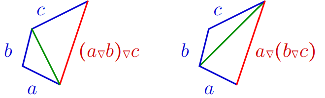
 .The role of zero is played by \(0\). The negation \(a\mapsto -a\) for
  is identity, as for any \(a\in \R _+\) the only real number \(x\) such that
  is \(a\).
 ![]()
Proof.
 .‘:Therefore
  .
.
 .
. ![]()
 appears in the representation theory. Denote by \(V^{(a)}\) the \(a\)th irreducible representation of \(sl_2\C \) (i.e., the symmetric power \(\Sym ^aV\) of the standard 2-dimensional representation \(V\)). Then the set
  parametrizes the set of irreducible representations of \(sl_2\C \) which are the summands in \(V^{(a)}\otimes V^{(b)}\):
5.2. Ultratriangle hyperfield.
The construction of Section 4.7 of hyperfield of linearly
ordered group, when applied to the multiplicative group of positive real numbers equipped with the usual order \(<\), defines a structure of hyperfield in \(\R _+\). Recall that the addition in this hyperfield is defined by formula
5.3. Tropical hyperfield.
The map \(\log :\R _{>0}\to \R \) is naturally extended by mapping \(0\) to \(-\infty \). The resulting map \(\R _+\to \R \cup \{-\infty \}\) is denoted also by \(\log \).
This is a bijection, and the hyperfield structure of \(\mfutr \) can be transferred via \(\log \) to \(\R \cup \{-\infty \}\). Denote the resulting hyperfield by \(\mftrop \), and call it the tropical hyperfield.
 , although
  .
.
5.4. Amoeba hyperfield.
Transfer via the same bijection \(\log :\R _+\to \R \cup \{-\infty \}\) the structure of the triangle hyperfield \(\mftr \) defined above in Section 5.1 to \(\R \cup \{-\infty \}\). The resulting hyperfield is called the amoeba hyperfield and denoted by \(\mfamb \).
5.6. Non-archimedian multiplicative seminorm.
Recall that a multiplicative seminorm \(K\to \R _+:x\mapsto |x|\) is non-archimedian if \(|x+y|\le \max (|x|,|y|)\). A non-archimedian multiplicative
seminorm \(K\to \R _+\) is a multiring homomorphism \(K\to \mfutr \). A non-archimedian valuation map, that is a composition of a non-archimedian multiplicative seminorm with \(\R _+\to \mftrop :x\mapsto \log x\), is a multiring homomorphism \(K\to
\mftrop \).
6. Tropical addition of complex numbers
6.1. Definition.
The tropical sum \(a\cplus b\) of arbitrary complex numbers \(a\) and \(b\) is defined as follows.
In formulas: if \(a=re^{\Ga i}\), \(b=re^{\Gb i}\) with \(|\Gb -\Ga |<\pi \), then \(a\cplus b=\{re^{\Gf i} \mid |\Ga -\Gf |+|\Gf -\Gb |=|\Ga -\Gb |\}\).
6.2. Obvious properties.
The tropical addition is commutative,
\(a\cplus b=b\cplus a\) for any \(a,b\in \C \). This follows immediately from the definition.
6.4. Distributivity.
![]()
Proof.
![]()
6.6. The tropical sum of several complex numbers.
The tropical sum of several complex numbers is affected only by those summands which have the greatest absolute value. A summand whose absolute values is
not maximal does not contribute at all.
Theorem 6.D.
Let \(a_1\), …, \(a_n\) be complex numbers with absolute values equal \(r\). Then
7. Relations of \(\tc \) with other hyperfields
7.1. Submultirings and subhyperfields.
Theorem 7.A.
Any subset \(A\) of \(\C \) containing \(0\),
invariant under the involution \(x\mapsto -x\) and closed with respect to multiplication inherits the structure of multiring from \(\tc \).
![]()
7.2. The tropical real hyperfield \(\tr \).
For example, \(\R \) inherits the structure of hyperfield. The induced addition \((a,b)\mapsto a\cplus _{\R }b=(a\cplus b)\cap \R \) can be described
directly as follows:
Proof.
![]()
7.3. The hyperfield of signs.
A structure of hyperfield comes in the same way to subsets \(A\subset \C \) which are not subfields of \(\C \). For example, \(\{-1,0,+1\}\subset \C \)
satisfies the conditions of Theorem 7.A , and hence inherits a hyperfield structure from \(\tc \). This hyperfield appeared above as \(\S \).
7.4. The phase hyperfield.
Let \(\Phi \) be \(\{z\in \C \mid |z|=1\}\cup \{0\}\), that is the unit circle in \(\C \) united with its center. This set satisfies the conditions of Theorem 7.A , and, by that theorem, \(\Phi \) inherits a hyperfield structure from \(\tc \). It will be called the phase hyperfield and denoted by \(\Phi \). One can obtain
\(\Phi \) also as \(\C /_m\R _{>0}\). Notice that \(\S =\Phi \cap \R \).
7.5. Embedding \(\T \subset \tc \).
Recall that a semifield is a set with two (univalued) operations, addition and multiplication, which satisfy all the axioms of field, except that there is no
subtraction.
7.6. The absolute value and amoeba maps.
The map \(\C \to \R _+:z\mapsto |z|\) is also a homomorphism from many points of view. This is
The composition of these maps with \(\log :\R _+\to \R \cup \{-\infty \}\) are the following multiring homomorphisms:
7.7. Complex polynomials and \(\tc \).
The map \(w\) which is defined and discussed in this section and the next one, essentially was defined by Mikhalkin [13] and used him in his definition of complex tropical curves. However, the algebraic properties of \(w\) were not considered, because the tropical addition of
complex numbers was not available.
Proof..
![]()
7.8. Real exponents.
The image of \(w\) consists of only those complex numbers whose absolute values are powers of \(e\). However similar constructions are able to provide multiring homomorphisms onto
the whole \(tc\). For this, it is enough to replace usual polynomials by polynomials with arbitrary real exponents.
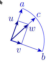
Figure 3. For given \(a,b,c\in \C \), constructing \(u,v,w\in \C \) such that \(A=uX^{r}\), \(B=vX^r\), \(C=wX^r\) with \(r=\log |a|\) and \(w(A)=a\), \(w(B)=b\), \(w(C)=c\), \(A+B=C\).
8. Continuity
8.1. Vietoris topologies.
The upper Vietoris topology in the set \(2^X\) of all subsets of a topological space \(X\) is the topology generated by the sets \(2^U\subset 2^X\), where \(U\) is open in \(X\). A neighborhood of a set
\(A\subset X\) in the upper Vietoris topology should contain all subsets of a set \(U\) that is open in \(X\) and contains \(A\).
8.2. Continuity and semi-continuities.
A multimap \(X\multimap Y\) is said to be
8.3. Tropical additions.
Proof.
![]()
Proof.
![]()
8.4. Continuity of triangle additions.
Recall that the triangle addition of non-negative real numbers is defined by formula  .
.
8.5. Properties of upper semi-continuous multimaps.
As we see above the additions in hyperfields \(\tc \), \(\tr \), \(\mftr \), \(\mfutr \), \(\mftrop \) and \(\mfamb \) are upper semi-continuous. Let \(K\)
denote one of these hyperfields.
Proof.
![]()
9. Dequantizations
9.1. The Litvinov-Maslov dequantization.
Consider a family of semirings \(\left \{S_h\right \}_{h\in [0,\infty )}\) (recall that a semiring is a sort of ring, but without subtraction). As a set, each of \(S_h\) is \(\R \). The
semiring operations \(+_h\) and \(\times _h\) in \(S_h\) are defined as follows:
\(\seteqnumber{0}{}{0}\)
9.2. Dequantization of the triangular hyperfield to the ultra-triangular.
For a positive real number \(h\), let \(R_h:\R _+\to \R _+\) be the map defined by formula \(x\mapsto x^{\frac 1h}\). This map is
invertible. Its inverse is defined by \(R_h^{-1}:x\mapsto x^h\).
 , then
 tend to the endpoints of the segment
  as \(h\to 0\). Define
  to be
to be  .
.
 and multiplication coinciding with the usual multiplication of real numbers. For \(h>0\), the map \(R_h\) is an isomorphism \(\mftr _h\to \mftr \). The hyperfield \(\mftr _0\) coincides with \(\mfutr \).
9.3. Dequantization of \(\C \) to \(\tc \).
For a positive real number \(h\), let \(S_h{:\ }\C \to \C \) be the map defined by the formula
 converges as \(h\) tends to zero. Namely:
 ;
;  ;
;  .
.
 as \(h\to 0\), but not in the sense of pointwise convergence.
Theorem 9.A.
Let \(\GG =\{(a,b,a+_hb,h)\in \C ^3\times \R _+\mid h>0, a\in \C ,b\in \C \}\). Then the intersection of \(\C ^3\times \{0\}\) with
the closure of \(\GG \) is the \(\GG _{\cplus }\times \{0\}\), where \(\GG _{\cplus }\) is the graph \(\{(a,b,a\cplus b)\mid a\in \C ,b\in \C \}\) of \((a,b)\mapsto a\cplus b\). Proof of
Theorem 9.A .
In the first case, if \(|a|>|b|\), then \(a=a+_0b\), hence \((a,b,a)\) belongs to the graph of \(+_0\), and therefore \((a,b,a,0)\) belongs to the closure of \(\GG \). If \(|a|<|b|\), then \(b=a+_0b\), hence \((a,b,b)\) belongs to the
graph of \(+_0\), and therefore \((a,b,b,0)\) belongs to the closure of \(\GG \).
Proof of Lemma 9.B .
![]()
Proof of Lemma 9.C .
![]()
Proof of Lemma 9.D .
![]()
Proof of Lemma 9.E .
![]()
![]()
9.4. Dequantizations commute.
We have constructed the following three 1-parameter families of hyperfields:
These families are related. The map \(\log :\R _+\to \R \cup \{-\infty \}\) maps the first of them to the second one. This is how the second deformation was obtained. Furthermore, the map \(\C \to \R _+:z\mapsto |z|\) maps the third deformation onto the first
one. The composition of these two maps, the amoeba map \(\C \to \R \cup \{-\infty \}:z\mapsto \log |z|\), maps the third deformation to the second one.
Appendix 1. Proof of Theorem 6.A
Let us prove that \((a\cplus b)\cplus c=a\cplus (b\cplus c)\) in each of these cases. In the framework of the prove in the case when \(x\cplus y\) is an arc (i.e., \(|x|=|y|\) and \(x+y\ne 0\)), let us denote this arc by \(\mathop \frown {(xy)}\).
![]()
![]()
![]()
![]()
![]()
![]()
![]()
Appendix 2. Proof of Theorem 6.D
![]()
Appendix 3. Other tropical additions
A3.1 Tropical addition of quaternions.
![]()
A3.2 Vector spaces over \(\tc \).
A3.3 Hyperfields of monomials.
![]()
![]()
![]()
![]()
![]()
![]()
A3.4 Tropical addition of \(p\)-adic numbers.
References
99
![\[ (a,b)\mapsto a\yplus b= \begin {cases} \max (a,b), &\text { if } a\ne b\\ \{x\in X\mid x\preceq a\}, &\text { if }a=b. \end {cases} \]](hf-images/image-7.svg)
![\[ (a,b)\mapsto a\upspoon b= \begin {cases} \max (a,b), &\text { if } a\ne b\\ \{x\in X\mid x\prec a\}, &\text { if }a=b\ne 0\\ 0, &\text { if }a=b=0. \end {cases} \]](hf-images/image-9.svg)
![\[ a\nplus b=\{c\in \R _+\mid |a-b|\le c\le a+b\}. \]](hf-images/image-32.svg)

![\[ 2\cdot 2\nplus 2\cdot 1\nplus 1\cdot 2\nplus 1\cdot 1=4\nplus 2\nplus 2\nplus 1 \]](hf-images/image-44.svg)
![\[ V^{(a)}\otimes V^{(b)}=\bigoplus _{c\in (a\nplus b)\cap (2\Z +a+b)}V^{(c)} \]](hf-images/image-48.svg)
![\[ (a,b)\mapsto a\yplus b= \begin {cases} \max (a,b), &\text { if } a\ne b\\ \{x\in \R _+\mid x\le a\}, &\text { if }a=b. \end {cases} \]](hf-images/image-49.svg)
![\[ (a,b)\mapsto a\yplus b= \begin {cases} \max (a,b), &\text { if } a\ne b\\ \{x\in \mftrop \mid x\le a\}, &\text { if }a=b. \end {cases} \]](hf-images/image-52.svg)
![\[ a\closedcurlyvee b=\{c\in \R \mid \log (|e^a-e^b|)\le c\le \log (e^a+e^b)\}, \]](hf-images/image-53.svg)
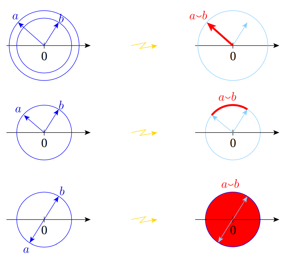
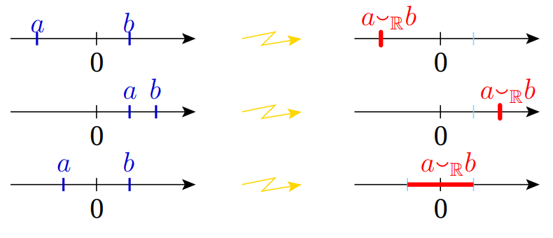
![\[ (a,b)\mapsto a\nplus b=\{c\in \R _+\mid |a-b|\le c\le a+b\}. \]](hf-images/image-55.svg)
![\[ a\nplus _h b=R_h^{-1}(R_h(a)\nplus R_h(b))= \{c\in \R _+\mid |a^{1/h}-b^{1/h}|^h\le c\le (a^{1/h}+b^{1/h})^h\}. \]](hf-images/image-56.svg)
![\[ \lim _{h\to 0}|a^{1/h}-b^{1/h}|^h=\lim _{h\to 0}(a^{1/h}+b^{1/h})^h=\max (a,b), \]](hf-images/image-58.svg)


![\[ a\cplus b = \begin {cases} \{a\}, &\text { if }\quad |a|>|b|;\\ \{b\}, &\text { if }\quad |a|<|b|;\\ \text {\parbox {2.3in}{ the set of points on the shortest geodesic arc connecting $a$ and $b$ in the sphere
$\{c\in \H \mid |c|=|a|\}$,}} &\text { if } |a|=|b|, \ a+b\ne 0\\ \text {the ball }\{c\in \H \mid |c|\le |a|\}, &\text { if }\quad a+b=0. \end {cases} \]](hf-images/image-71.svg)