(Semi-) Parabolic Implosion

Processing math: 47%

(Semi-) Parabolic Implosion

Does the Julia set depend continuously on the polynomial?

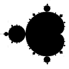
Let us start in dimension one and consider the quadratic family

$q_c(z) = z^2+c$ . The bifurcation locus for the family

$\{q_c:c\in{\Bbb C}\}$ is given by the boundary of the Mandelbrot set

$M$ . The largest "bubble" of

$M$ is the "main cardiod".

We can ask: Is the map $c\mapsto J_c$ continuous? Douady has given an answer:
If $c_0$ is a point on the boundary of the main cardioid, then $c\mapsto J_c$ is continuous at $c_0$ if and only if $c_0$ is not a parabolic parameter, i.e., if $q_{c_0}$ does not have a periodic cycle which is parabolic.

We recall that a point

$z_0$ is periodic if

$q^n_{c}(z_0)=z_0$ , and a periodic point is parabolic if

$(q_c^n)'(z_0)$ is a root of unity. The parabolic points on the boundary of the main cardioid are the points where one of the (infinitely many) "bubbles" attach, together with the most conspicuous of the parabolic points,

$c=\frac{1}{4}$ , which is the cusp point.
The point

$z_0=\frac 1 2$ is fixed by

$q_{{\frac 1 4}}$ , and

$q_{\frac 1 4}'(z_0)=1$ , so this is parabolic. It has been proved that:
The Julia set $J_c$ varies continuously if we move $c$ to the left: i.e., $J_{\frac1 4 - t}$ is continuous for $0\le t\le \frac1 4$ .

The situation is more complicated when

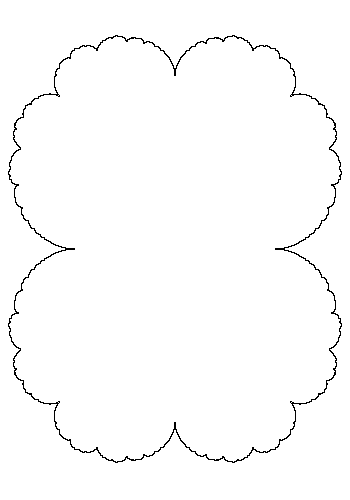
$c>\frac 1 4$ . The figures below show how the Julia sets

$J_{\frac 1 4 + \epsilon}$ evolve as

$\epsilon$ decreases to 0 (as we move from right to left).

Julia sets

$J_{\frac 1 4 + \epsilon}$ : "Cauliflower" (

$\epsilon=0$ ) on left;

$\epsilon=.0005$ in center;

$\epsilon=.01$ on right.

We can see that

$J_{\frac1 4 +.0005}$ looks somewhat like

$J_{\frac 1 4}$ from the "outside", but on the "inside" there are curlicues; pairs of them are vaguely reminiscent of "butterflies". As

$t\to0$ , these butterflies persist and remain uniformly large. We think of

$t$ as representing time, which decreases to 0. The fact that they suddenly disappear for

$t=0$ is the phenomenon called "implosion". Or, if we think of time starting at

$t=0$ , then the instantaneous appearance of large "butterflies" for

$t>0$ may be thought of as "explosion".

Semi-parabolic fixed points.

We consider the family of complex Hénon maps

$f:{\Bbb C}^2\to{\Bbb C}^2$ given by

$f_{a,c}(x,y) = (x^2+c-a y, x). \ \ \ \ \ \ (1)$ The fixed points are

$p_0=(t,t)$ with

$t^2 -(1+a)t + c=0$ . If

$(a+1)^2 =4c, \ \ \ \ \ \ \ \ \ \ \ (2)$ then

$p_0$ is semi-parabolic, which means that the eigenvalues of

$Df(p_0)$ are 1 and

$a$ . We assume that

$0<|a|< 1$ , and thus

$p_0$ is also semi-attracting. If we translate the fixed point to the origin

$O=(0,0)$ , then our map takes the form

$f(x,y)=(x+x^2+\cdots, ay + \cdots)$ where the "

$\cdots$ " indicates terms in

$(x,y)$ which are higher order. The semi-parabolic basin

${\cal B}:=\{p\in{\Bbb C}^2: \lim_{n\to\infty}f^n=O \text{ uniformly in a neighborhood of }p\}$ In fact, Ueda has shown that there is an Abel-Fatou function

$\Phi_{AF}:{\cal B}\to {\Bbb C}$ , satisfying

$\Phi_{AF}(f) = \Phi_{AF}+1$ .
The counterpart to

${\cal B}$ for negative time is the asymptotic curve

$\Sigma:= \{p\in{\Bbb C}^2: p\ne O, \lim_{n\to\infty}f^{-n}(p)=O \}$ As the counterpart for Abel-Fatou function, Ueda has shown that there is a uniformization

$H:{\Bbb C}\to \Sigma$ such that

$f( H(\zeta)) = H(\zeta+1)$ for all

$\zeta\in{\Bbb C}$ .

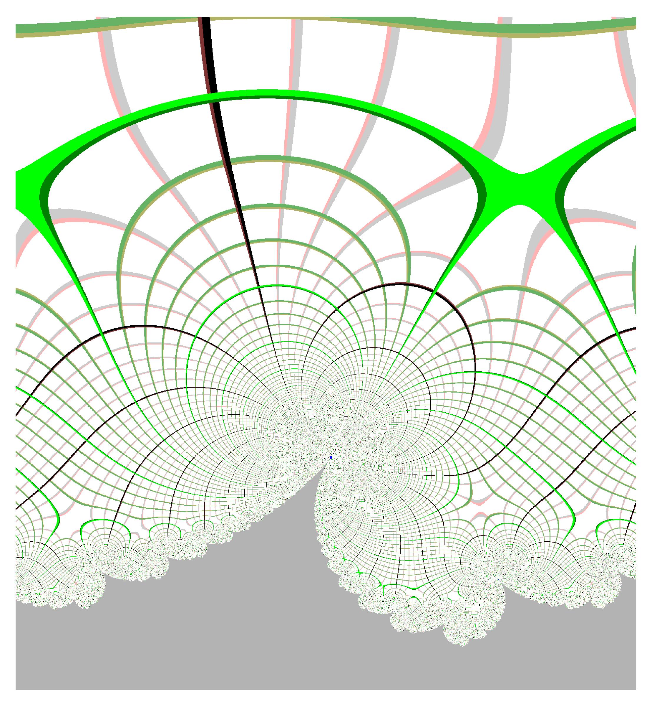
A natural way to represent the basin

${\cal B}$ is to draw the intersection

${\cal B}\cap \Sigma$ in terms of the Fatou coordinate

$H$ . For instance, for

$a = .15$ (and

$c$ chosen according to (2)), we find the picture at left. By the Abel-Fatou property, the whole picture is invariant under translation to the right (adding

$+1$ ). The gray region is the complement

${\Bbb C}^2-{\cal B}$ , and the rest is

${\cal B}$ . We can observe cusps in the boundary that are reminiscent of the cusps in the "Cauliflower" Julia set. The green lines are level sets of the imaginary part of

$\Phi_{AF}$ , and the pink/gray lines are level sets of the real part. These level sets form rectangles in much of the picture. Where they form octagons, there must be a critical point of

$\Phi_{AF}$ inside. Also, the large green "X" indicates a critical point.

Does the Julia set vary continuously with the map?

For complex Hénon maps, there are both a forward Julia set

$J^+$ (for

$f$ ) and a backward Julia set

$J^-$ (the forward Julia set for

$f^{-1}$ ). We define:

$J:=J^+\cap J^-$ . It is known that if

$f$ is a hyperbolic Hénon map, then

$f$ is structurally stable, which means that

$f|_{J_f}$ is conjugate to

$\tilde f_{J_{\tilde f}}$ for

$\tilde f$ close to

$f$ . Further, and

$J_f$ depends continuously on

$f$ . In general, this fails in the non-hyperbolic case. However, in the semi-parabolic case, there is an interesting paper of R. Radu and R. Tanase where it is shown:

Suppose that $a$ and $c$ satisfy (2) above, and let $f_{a,c}$ be as in (1). Then for sufficiently small $|a|>0$ , the sets $J_{a,c}$ are all homeomorphic and vary continuously. In fact, the restrictions of these maps, $f_{a,c}|_{J_{a,c}}$ , are conjugate to each other.

Semi-parabolic implosion in ${\Bbb C}^2$

Now we perturb the map (1) as follows. We consider the parameters

$(a,c)$ to be fixed, and for

$\epsilon\ne0$ , we consider

$f_\epsilon(x,y) = (\epsilon^2+x+x^2+\cdots, ay+\cdots)$ After such a pertubation, we expect condition (2) to be lost. For

$\epsilon=0$ , the fixed point

$O$ had multiplicity 2, and one of the multipliers is 1. For

$\epsilon>0$ is splits into a pair of fixed points, and the multiplier 1 splits into a pair of multipliers which are approximately

$1\pm i\epsilon$ . In this paper written with Smillie and Ueda, we show that a semi-parabolic phenomenon takes place, very much like the parabolic implosion situation in

${\Bbb C}$ , which we described above. This paper is a revision of the paper we put on the arXiv several years ago.

In order to have pictures in

${\Bbb C}^2$ , which has real dimension 4, we cannot simply draw pictures like the "Cauliflower" above. Thus we draw pictures inside the slice by

$\Sigma$ .

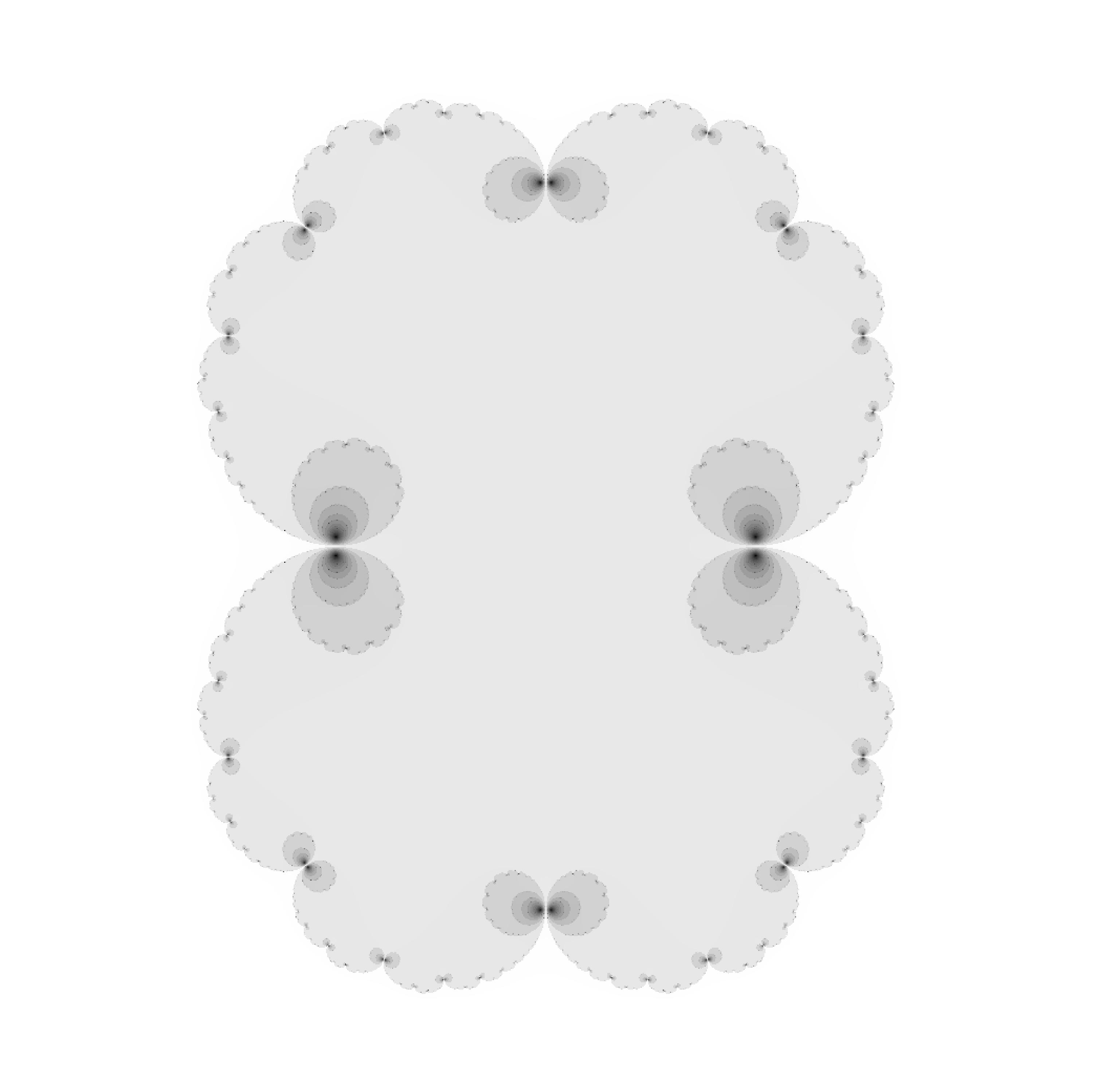
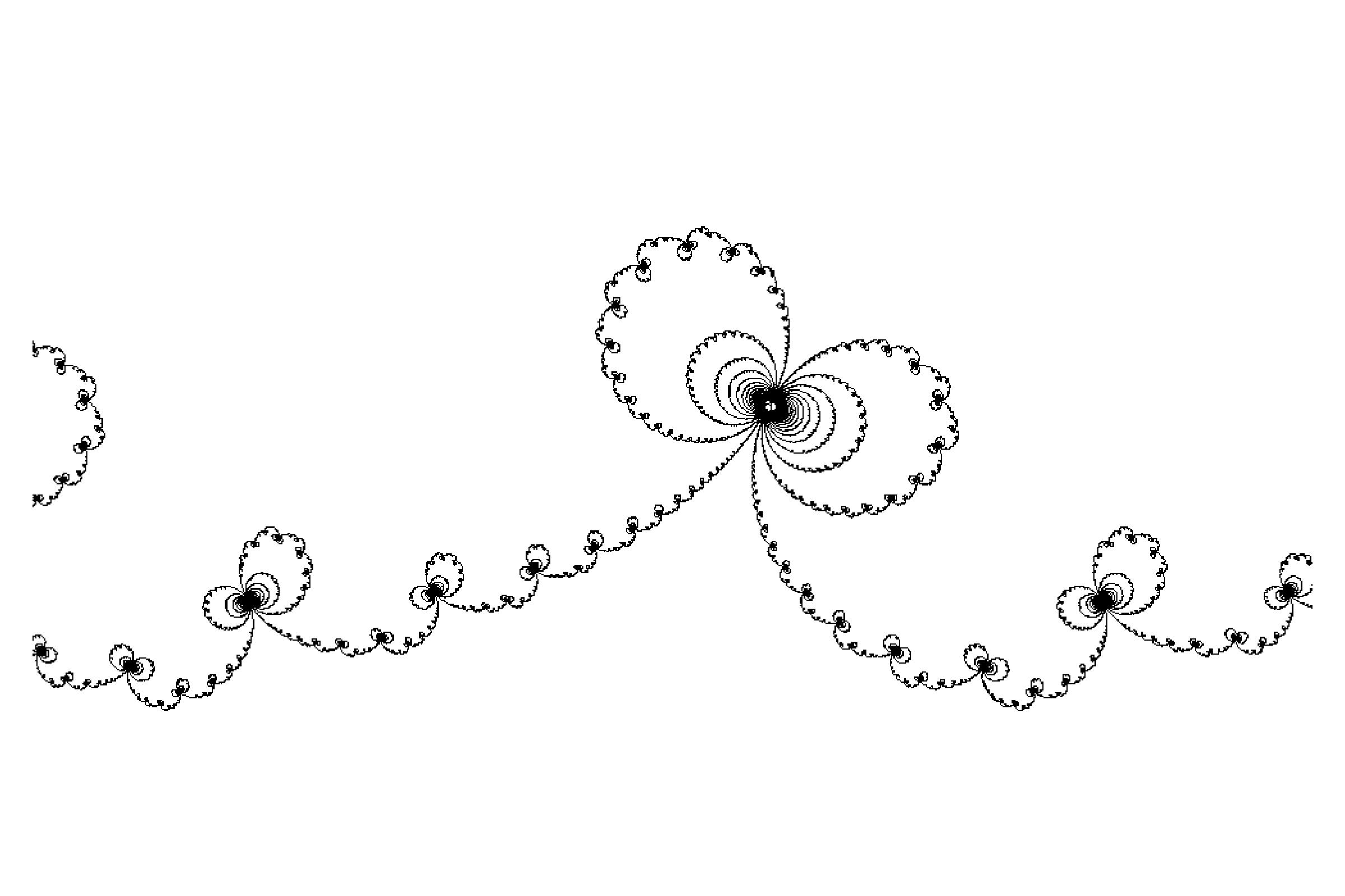
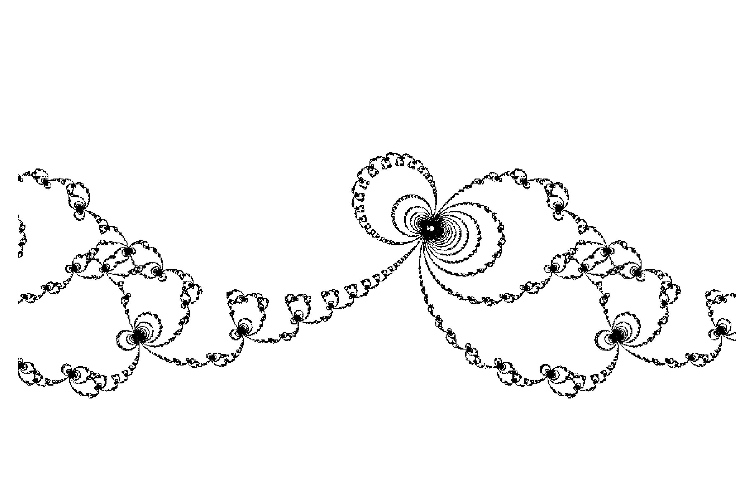
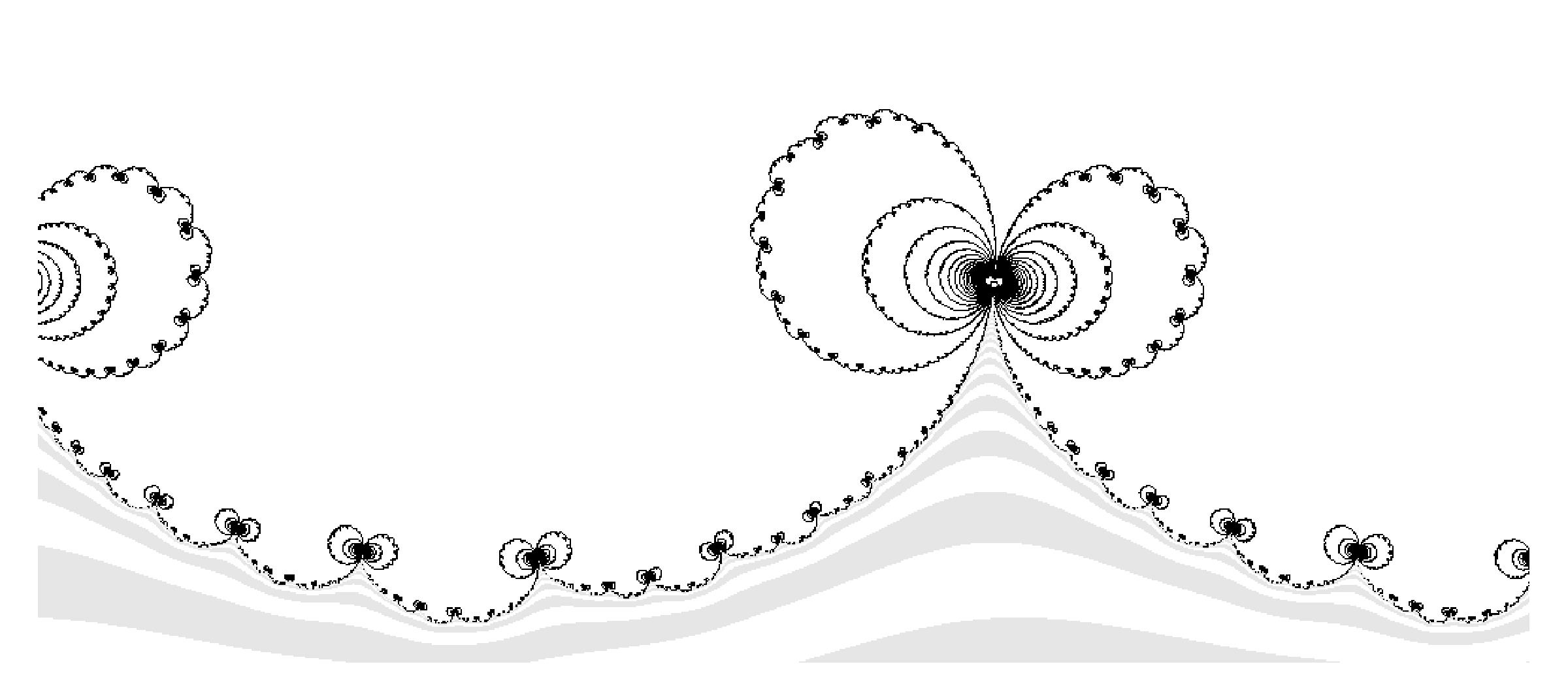
As examples of the "curlicues" that arise in the "butterflies" we have pictures like the ones on the right. These pictures are invariant under horizontal translation

$\zeta\mapsto\zeta+1$ and represent maps of the form (1) with

$a$ and

$c$ satisfying (2).

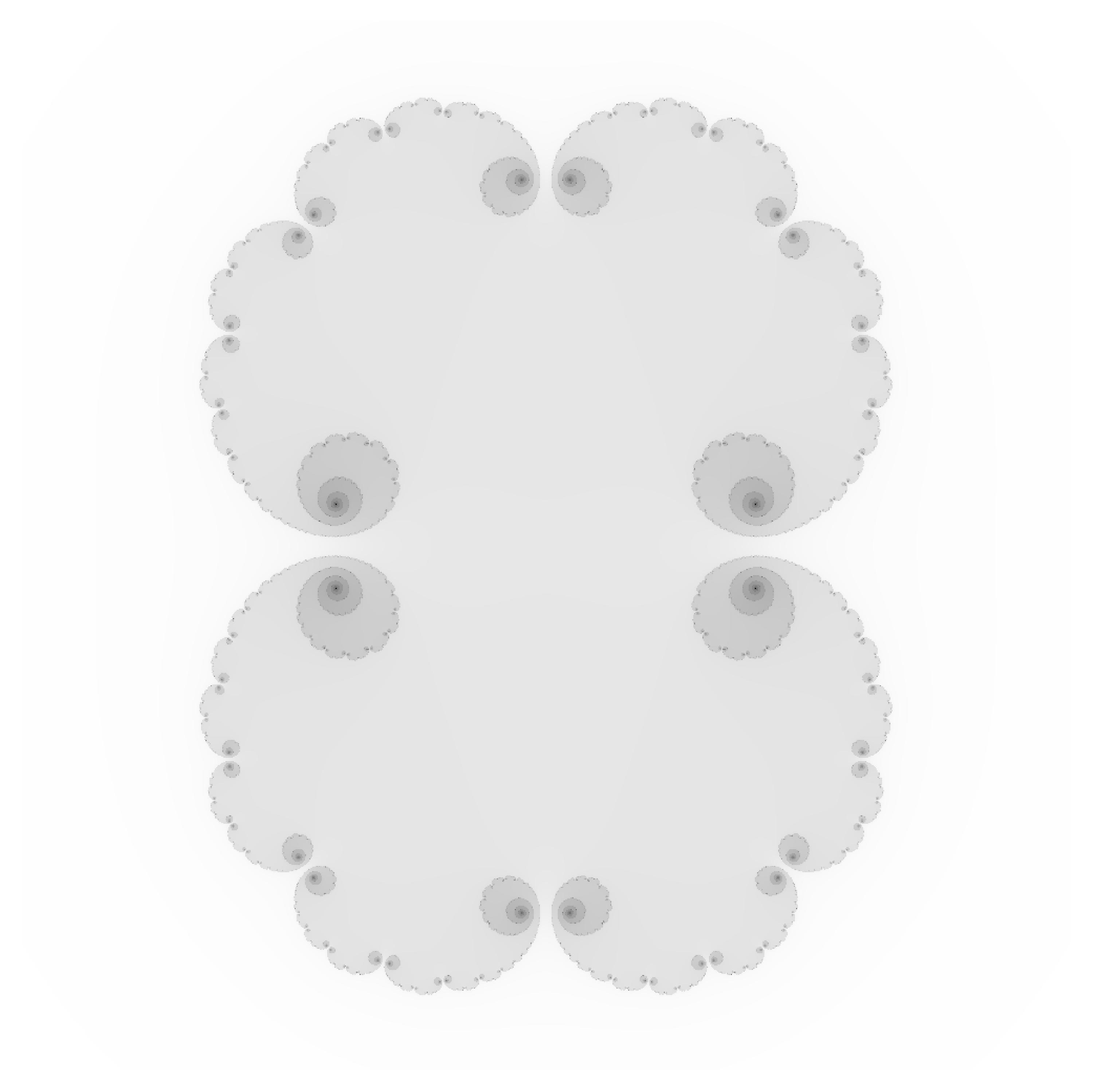
In the first two pictures, we have

$a=.1$ The bottoms of these pictures show the boundary

$(\partial{\cal B})\cap\Sigma$ , which can be seen to be the same in both cases. The difference in the "curlicues" arises because

$\epsilon\to0$ along different paths. The color pictures on the main page also show examples of imploded sets.

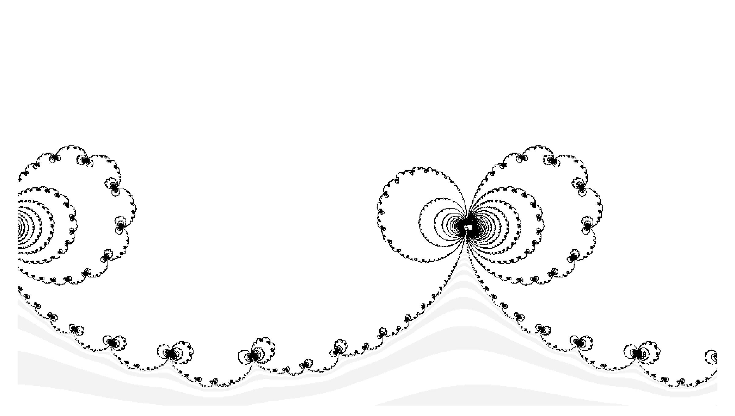
We have

$a=.1\sqrt{-1}$ in the next two pictures. The alternating gray/white indicates the complement of

${\cal B}$ . (The alternating white/gray was not displayed when the first two pictures were made.)

To go back to the main page click here.