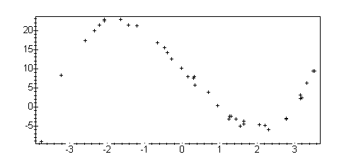
Let's now try to fit a cubic polynomial to some data. Again, maple's built-in package can do this for us, but we like to work harder than we need to, so we understand more. First, lets read some data in from a file, and take a look at it.
cubdata := read('cubdata.maple'):
plot(pts,style=point, axes=boxed);

As in the linear case, we will do the work "by hand".
To simplify typing, let's define the type of function we want to fit. We know (somehow) that our goal is to fit a monic cubic polynomial, so
cub := (x,a,b,c) ->  x^3 + a*x^2 + b*x + c;

                                      3      2
              cub := (x, a, b, c) -> x  + a x  + b x + c
Now we define an "error functional" which gives us the distance from our cubic to our data. Note that we use maple's "nops" command so that we don't need to explicitly say how many points there are.
G := (a,b,c) -> sum((cub(pts[i][1],a,b,c) - pts[i][2] )^2,
                    i=1..nops(pts));

                    nops(pts)
                      -----
                       \                                           2
  G := (a, b, c) ->     )     (cub(pts[i][1], a, b, c) - pts[i][2])
                       /
                      -----
                      i = 1
Now we just ask maple to find the (unique) critical point of G, which is our minimum. Since we used assign to set the coefficients, we won't see a result.
assign(solve( {diff( G(a,b,c), a)=0,
               diff( G(a,b,c), b)=0,
               diff( G(a,b,c), c)=0},
             {a,b,c} ));
but we can readily see what the answer is:
cub(x,a,b,c);

           3                2
          x  - .4806519894 x  - 10.94459406 x + 10.28284644
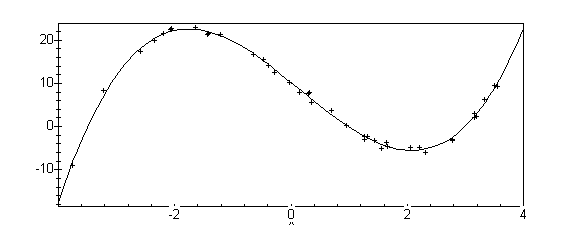
Finally, lets make a picture, just to see how well it fits
with(plots):
cplot := plot(cub(x,a,b,c), x=-4..4, axes=boxed):
pplot:= plot(pts, style=point):
display({cplot, pplot});
