MAT131 - Project 1
A Solution

In this project, we are to model the population growth of kafit birds in the Greater Boomchalaka game preserve. The populations were tabulated in several years as shown in the table below.

year	0	1	5	6
# birds	470	940	25,220	93,590

1. We are to find the cubic polynomial C(x) = a x³ + b x² + c x + d that goes through all four of the data points, then use this to estimate the population of kafit birds in years 2, 3, and 4.

Since the polynomial is required to pass through the given points, each of the points must satisfy the functional relationship. Thus, whatever a, b, c, and d are, the following equations must all be true.

$$\begin{array}{rcrcrcrcr} 470 & = C(0) = & && && && d \\ 94... ... 93590 & = C(6) = & 216a &+& 36b &+& 6c &+& d \\ \end{array}$$

We need to solve these equations simultaneously. There are many different schemes for doing this, although at some level they are all the same thing. We will just solve an equation for one variable in terms of the others, and substitute that into the next equation. Other methods may be more efficient, but this way is completely straightforward.

From C(0), we see immediately that d=470. Substituting into the next equation, we see that

C(1) = a+b+c+470 = 940

so we have c = 470 - a -b. Substituting into the equation for C(5), we get

25220 = 125a + 25b + 5(470 - a - b) + 470 = 120a +20b +2820

or, equivalently, b = 1120 - 6a. Putting this in the last line,

93590 = 216a + 36(1120 - 6a) + 6(470 - a -[470-a-(1120 - 6a)]) +470,

so, after simplifying, 30a = 56700. This means that

$$a=1890, \qquad b=-10220, \qquad c=880, \qquad{\rm and}\quad d=470.$$

Thus, our desired polynomial is

C(x) = 1890x³ - 10220x² + 880x + 470.

If C(x) described the population of kafit birds exactly, then plugging in the year for x should give us the population in that year.

year		population	comment
0	C(0) = 470	470	Matches our data
1	C(1) = 1890 - 10220 + 8800 + 470	940	Matches our data
2	C(2) = 15120 - 40880 + 17600+ 470	-7690	A negative population
3	C(3) = 51030 - 91980 + 26400 + 470	-14080	Also negative
4	C(4) = 120960 -163520 +35200 + 470	-6890	Still negative
5	C(5) = 236250 -255500 +44000 + 470	25220	Matches again
6	C(6) = 408240 -367920 +52800 + 470	93590	also OK

Here is a graph of C(x), with the known populations marked by circles. Note that it passes through each of them, but is negative from early in year 1 until the beginning of year 4.

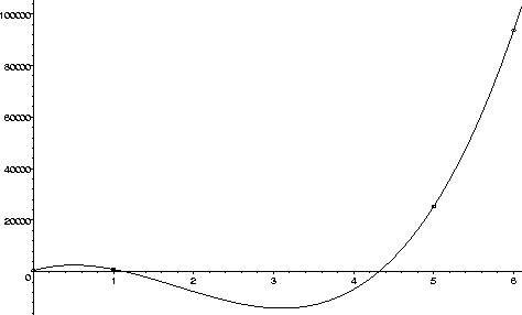
This seems a little suspect as a description of bird populations, but everything was done correctly. Note that all the populations were were given match the values of C(x), but the predicted populations for years 2, 3, and 4 are negative, which is not physically possible. So it seems very unlikely that C(x) is a good choice of model for the population of kafit birds.

We could try to find a more reasonable cubic polynomial by relaxing the requirement that our model polynomial pass exactly through all the points. This is not an unreasonable thing to do, since the model is only intended to approximate the given data, not match it exactly. Also, the population counts are probably inexact, as well.

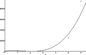
However, in order to get a cubic polynomial which stays positive, I had to adjust the population counts by approximately 25%. For example, using the data points (0,470), (1,1175), (5,32000), and (6,70000), we obtain the cubic polynomial $\frac{9317}{12}x^3 - \frac{13033}{4}x^2 + \frac{19121}{6}x + 470$which gives us estimated populations of 22, 1669.5, and 10776 in years 2, 3, and 4. The graph is shown below.

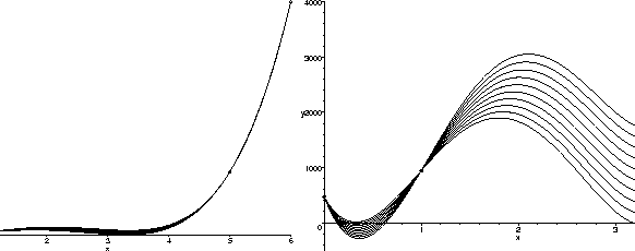
Another possibility is to use a higher degree polynomial. If we estimate (somewhat arbitrarily) a value for the population in, say, year 3, we can perform the same procedure as before to find the unique fourth degree polynomial which passes through all 5 of the given points. On the left below are the graphs of the polynomials resulting from 10 such choices. The general shape seems almost reasonable, look at the magnification of the graphs for 0 < x < 4 on the right. Note that while the population estimates which result are all positive, the shape of the graph is less than fully satisfying. The functions drop dramatically in the first and third years.

We could, of course, use an even higher degree polynomial to try to get a shape that matches better with our intuition. However, the whole process is beginning to seem quite artificial. The problem is that the shape of a low-degree polynomial is just too restrictive to model this data well.

2. For the second part, we try to find an exponential function $E(x) = k\,e^{ax}$ that models the data, and use it to estimate the population in years 2, 3, and 4.

Because E(x) depends only on two numbers k and a, we can only force it to pass exactly through two of our data points. We can, however, try to make it come as close as possible to the others.

First, it seems reasonable to assume that the population for year 0 is exact, and the other years may contain counting errors, because we should know exactly how many birds were resettled, but counting birds in the wild can be a tricky, inexact process. If we make this assumption, we have $E(0) = k\,e^0$, and so we must have k=470.

To find the value of a, we can pick any one of the other data points, and solve. Let's use (5, 25220) to illustrate the process.

Plugging in, we have

E(5) = 25220 = 470 e^5a

and so

$$e^{5a} = \frac{2522}{47}.$$

We can take the logarithm of both sides of the equation to obtain

$$5a = \ln \left( \frac{2522}{47} \right) \qquad{\rm so}\qquad ... ...\frac{1}{5}\ln \left( \frac{2522}{47} \right) \approx 0.79653$$

This gives $E_5(x) = 470 e^{\frac{x}{5}\ln\frac{2522}{47}} \approx 470e^{0.79653x}$as our function.

It should be pretty clear that if we had used one of the other points instead, we should get either $E_1(x) = 470 e^{x\ln 2} \approx 470 e^{0.69315x}$or $E_6(x) = 470 e^{\frac{x}{6}\ln\frac{9359}{47}} \approx 470e^{0.88232x}$.

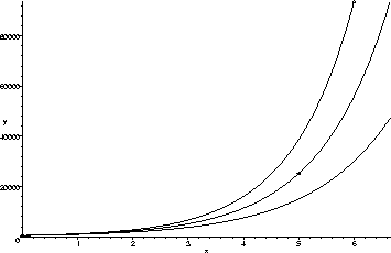
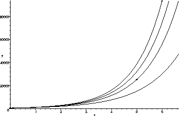
The graphs of all three are shown above. The best of the three seems to be E₅ (the one in the middle). Using E₅ to estimate the bird populations in years 2, 3, and 4, we obtain 2311, 5127, and 11371, respectively. Note that E₅ gives a population of 1042 in year 1 and 55934 in year 6. These are relative errors of about 20% and 40%-- not so great.

Of course, there is no reason we need go through any of the points exactly. We could just play around with the values of a and k until we got something that looks better, or pick a pair of points that seem ``sort of in the middle'' and repeat the process above, or we could average the points or the exponents in some way. However, there is another way. Note that if we take the logarithm of E(x), we get

$$\ln\left(E(x)\right) = \ln k + \ln \left( e^{ax} \right) = \ln k + ax$$

Since k is an unknown constant, its logarithm is just another (positive) constant. This means that the logarithm of E(x) is a straight line. We can try to find the line that comes closest to the points whose x coordinate is the year, and whose y coordinate is the logarithm of the population in that year.

Taking the natural logarithm of the populations, we get the data to fit as

$$(0,6.15273),\, (1, 6.84587),\, (5, 10.13539),\, (6,11.44667).$$

One way to find the line which comes nearest all of these points is to use linear regression; this process finds the line that minimizes the sum of the squares of the distance to the points. Your calculator probably has the ability to do linear regression built into it; the theory behind how it works will come later in the calculus sequence. (Rather than using regression, you could just plot a graph and ``eyeball'' the solution, and do a very good job).

Using regression, the best fit line is found to be

y = 0.86388 x + 6.05353

Exponentiating this line gives us

$$E(x) = 425.614 \, e^{ 0.86388 x},$$

which gives kafit bird populations of 426, 1010, 2395, 5683, 13481, 31982, and 75872 for each of the years. This is less than 20% relative error for the known data, and isn't too bad. The graph of the exponential is shown below, along with the three we found above for comparison. The graph of the exponential found by regression is shown as the thickest of the four (just below the top one).

We should remark that with so little information (only four points), making a good model is nearly impossible. Even with sufficient data, modelling can be a very tricky business.