Patchworking real algebraic varieties
oleg.viro@@gmail.com
1991 Mathematics Subject Classification:
14G30, 14H99; Secondary 14H20, 14N10Introduction
This paper is a translation of the first chapter of my dissertation 11This is not a Ph D., but a dissertation for the degree of Doctor of Physico-Mathematical Sciences. In Russia there are two degrees in mathematics. The lower, degree corresponding approximately to Ph D., is called Candidate of Physico-Mathematical Sciences. The high degree dissertation is supposed to be devoted to a subject distinct from the subject of the Candidate dissertation. My Candidate dissertation was on interpretation of signature invariants of knots in terms of intersection form of branched covering spaces of the 4-ball. It was defended in 1974. which was defended in 1983. I do not take here an attempt of updating.
The results of the dissertation were obtained in 1978-80, announced in [Vir79a]; [Vir79b]; [Vir80], a short fragment was published in detail in [Vir83a] and a considerable part was published in paper [Vir83b]. The later publication appeared, however, in almost inaccessible edition and has not been translated into English.
In [Vir89] I presented almost all constructions of plane curves contained in the dissertation, but in a simplified version: without description of the main underlying patchwork construction of algebraic hypersurfaces. Now I regard the latter as the most important result of the dissertation with potential range of application much wider than topology of real algebraic varieties. It was the subject of the first chapter of the dissertation, and it is this chapter that is presented in this paper.
In the dissertation the patchwork construction was applied only in the case of plane curves. It is developed in considerably higher generality. This is motivated not only by a hope on future applications, but mainly internal logic of the subject. In particular, the proof of Main Patchwork Theorem in the two-dimensional situation is based on results related to the three-dimensional situation and analogous to the two-dimensional results which are involved into formulation of the two-dimensional Patchwork Theorem. Thus, it is natural to formulate and prove these results once for all dimensions, but then it is not natural to confine Patchwork Theorem itself to the two-dimensional case. The exposition becomes heavier because of high degree of generality. Therefore the main text is prefaced with a section with visualizable presentation of results. The other sections formally are not based on the first one and contain the most general formulations and complete proofs.
In the last section another, more elementary, approach is expounded. It gives more detailed information about the constructed manifolds, having not only topological but also metric character. There, in particular, Main Patchwork Theorem is proved once again.
I am grateful to Julia Viro who translated this text.
1. Patchworking plane real algebraic curves
This Section is introductory. I explain the character of results staying in the framework of plane curves. A real exposition begins in Section 2. It does not depend on Section 1. To a reader who is motivated enough and does not like informal texts without proofs, I would recommend to skip this Section.
1.1. The case of smallest patches
We start with the special case of the patchworking. In this case the patches are so simple that they do not demand a special care. It purifies the construction and makes it a straight bridge between combinatorial geometry and real algebraic geometry.
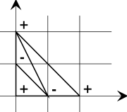
1.1.A Initial Data.
Let $m$ be a positive integer number [it is the degree of the curve under construction]. Let $\Delta$ be the triangle in ${\bf R}^{2}$ with vertices $(0,0)$, $(m,0)$, $(0,m)$ [it is a would-be Newton diagram of the equation]. Let $\mathcal{T}$ be a triangulation of $\Delta$ whose vertices have integer coordinates. Let the vertices of $\mathcal{T}$ be equipped with signs; the sign (plus or minus) at the vertex with coordinates $(i,j)$ is denoted by $\sigma_{i,j}$.
See Figure 1.
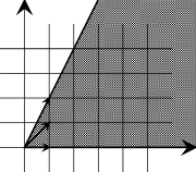
For $\varepsilon,\delta=\pm 1$ denote the reflection ${\mathbb{R}}^{2}\to{\mathbb{R}}^{2}:(x,y)\mapsto(\varepsilon x,\delta y)$ by $S_{\varepsilon,\delta}$. For a set $A\subset{\mathbb{R}}^{2}$, denote $S_{\varepsilon,\delta}(A)$ by $A_{\varepsilon,\delta}$ (see Figure 2). Denote a quadrant $\{(x,y)\in{\mathbb{R}}^{2}\,|\,\varepsilon x>0,\delta y>0\}$ by $Q_{\varepsilon,\delta}$.

The following construction associates with Initial Data 1.1.A above a piecewise linear curve in the projective plane.
1.1.B Combinatorial patchworking.
Take the square $\Delta_{*}$ made of $\Delta$ and its mirror images $\Delta_{+-}$, $\Delta_{-+}$ and $\Delta_{--}$. Extend the triangulation $\mathbb{T}$ of $\Delta$ to a triangulation $\mathbb{T}_{*}$ of $\Delta_{*}$ symmetric with respect to the coordinate axes. Extend the distribution of signs $\sigma_{i,j}$ to a distribution of signs on the vertices of the extended triangulation which satisfies the following condition: $\sigma_{i,j}\sigma_{\varepsilon i,\delta j}\varepsilon^{i}\delta^{j}=1$ for any vertex $(i,j)$ of $\mathbb{T}$ and $\varepsilon,\delta=\pm 1$. (In other words, passing from a vertex to its mirror image with respect to an axis we preserve its sign if the distance from the vertex to the axis is even, and change the sign if the distance is odd.)22More sophisticated description: the new distribution should satisfy the modular property: $g^{*}(\sigma_{i,j}x^{i}y^{j})=\sigma_{g(i,j)}x^{i}y^{j}$ for $g=S_{\varepsilon\delta}$ (in other words, the sign at a vertex is the sign of the corresponding monomial in the quadrant containing the vertex).
If a triangle of the triangulation $\mathbb{T}_{*}$ has vertices of different signs, draw the midline separating the vertices of different signs. Denote by $L$ the union of these midlines. It is a collection of polygonal lines contained in $\Delta_{*}$. Glue by $S_{--}$ the opposite sides of $\Delta_{*}$. The resulting space $\bar{\Delta}$ is homeomorphic to the projective plane ${\mathbb{R}}P^{2}$. Denote by $\bar{L}$ the image of $L$ in $\bar{\Delta}$.

Let us introduce a supplementary assumption: the triangulation $\mathbb{T}$ of $\Delta$ is convex. It means that there exists a convex piecewise linear function $\nu:\Delta\to{\mathbb{R}}$ which is linear on each triangle of $\mathbb{T}$ and not linear on the union of any two triangles of $\mathbb{T}$. A function $\nu$ with this property is said to convexify $\mathbb{T}$.
In fact, to stay in the frameworks of algebraic geometry we need to accept an additional assumption: a function $\nu$ convexifying $\mathbb{T}$ should take integer value on each vertex of $\mathbb{T}$. Such a function is said to convexify $\mathbb{T}$ over ${\mathbb{Z}}$. However this additional restriction is easy to satisfy. A function $\nu:\Delta\to{\mathbb{R}}$ convexifying $\mathbb{T}$ is characterized by its values on vertices of $\mathbb{T}$. It is easy to see that this provides a natural identification of the set of functions convexifying $\mathbb{T}$ with an open convex cone of ${\mathbb{R}}^{N}$ where $N$ is the number of vertices of $\mathbb{T}$. Therefore if this set is not empty, then it contains a point with rational coordinates, and hence a point with integer coordinates.
1.1.C Polynomial patchworking.
Given Initial Data $m$, $\Delta$, $\mathbb{T}$ and $\sigma_{i,j}$ as above and a function $\nu$ convexifying $\mathbb{T}$ over ${\mathbb{Z}}$. Take the polynomial
| $b(x,y,t)=\sum_{{\small\begin{aligned}&\displaystyle(i,j)\text{\enspace runs % over}\\ &\displaystyle\text{\quad vertices of $\mathbb{T}$}\end{aligned}}}\sigma_{i,j}% x^{i}y^{j}t^{\nu(i,j)}.$ |
and consider it as a one-parameter family of polynomials: set $b_{t}(x,y)=b(x,y,t)$. Denote by $B_{t}$ the corresponding homogeneous polynomials:
| $B_{t}(x_{0},x_{1},x_{2})=x_{0}^{m}b_{t}(x_{1}/x_{0},x_{2}/x_{0}).$ |
1.1.D Patchwork Theorem.
Let $m$, $\Delta$, $\mathbb{T}$ and $\sigma_{i,j}$ be an initial data as above and $\nu$ a function convexifying $\mathbb{T}$ over ${\mathbb{Z}}$. Denote by $b_{t}$ and $B_{t}$ the non-homogeneous and homogeneous polynomials obtained by the polynomial patchworking of these initial data and by $L$ and $\bar{L}$ the piecewise linear curves in the square $\Delta_{*}$ and its quotient space $\bar{\Delta}$ respectively obtained from the same initial data by the combinatorial patchworking.
Then there exists $t_{0}>0$ such that for any $t\in(0,t_{0}]$ the equation $b_{t}(x,y)=0$ defines in the plane ${\mathbb{R}}^{2}$ a curve $c_{t}$ such that the pair $({\mathbb{R}}^{2},c_{t})$ is homeomorphic to the pair $(\Delta_{*},L)$ and the equation $B_{t}(x_{0},x_{1},x_{2})=0$ defines in the real projective plane a curve $C_{t}$ such that the pair $({\mathbb{R}}P^{2},C_{t})$ is homeomorphic to the pair $(\bar{\Delta},\bar{L})$.
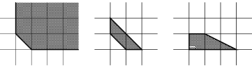
Example 1.1.E .
Construction of a curve of degree 2 is shown in Figure 3. The broken line corresponds to an ellipse. More complicated examples with a curves of degree 6 are shown in Figures 4, 5.


For more general version of the patchworking we have to prepare patches. Shortly speaking, the role of patches was played above by lines. The generalization below is a transition from lines to curves. Therefore we proceed with a preliminary study of curves.
1.2. Logarithmic asymptotes of a curve
As is known since Newton’s works (see [New67]), behavior of a curve $\{(x,y)\in{\mathbb{R}}^{2}\,|\,a(x,y)=0\}$ near the coordinate axes and at infinity depends, as a rule, on the coefficients of $a$ corresponding to the boundary points of its Newton polygon $\Delta(a)$. We need more specific formulations, but prior to that we have to introduce several notations and discuss some notions.
For a set $\Gamma\subset{\mathbb{R}}^{2}$ and a polynomial $a(x,y)=\sum_{\omega\in\mathbb{Z}^{2}}a_{\omega}x^{\omega_{1}}y^{\omega_{2}}$, denote the polynomial $\sum_{\omega\in\Gamma\cap\mathbb{Z}^{2}}a_{\omega}x^{\omega_{1}}y^{\omega_{2}}$ by $a^{\Gamma}$. It is called the $\Gamma$-truncation of $a$.
For a set $U\subset{\mathbb{R}}^{2}$ and a real polynomial $a$ in two variables, denote the curve $\{(x,y)\in U\,|\,a(x,y)=0\}$ by $V_{U}(a)$.
The complement of the coordinate axes in ${\mathbb{R}}^{2}$, i.e. a set $\{(x,y)\in{\mathbb{R}}^{2}\,|\,xy\not=0\}$, is denoted33This notation is motivated in Section 2.3 below. by ${\mathbb{R}}{\mathbb{R}}^{2}$.
Denote by $l$ the map ${\mathbb{R}}{\mathbb{R}}^{2}\to{\mathbb{R}}^{2}$ defined by formula $l(x,$ $y)=(\ln|x|,\ln|y|)$. It is clear that the restriction of $l$ to each quadrant is a diffeomorphism.
A polynomial in two variables is said to be quasi-homogeneous if its Newton polygon is a segment. The simplest real quasi-homogeneous polynomials are binomials of the form $\alpha x^{p}+\beta y^{q}$ where $p$ and $q$ are relatively prime. A curve $V_{\mathbb{RR}^{2}}(a)$, where $a$ is a binomial, is called quasiline. The map $l$ transforms quasilines to lines. In that way any line with rational slope can be obtained. The image $l(V_{\mathbb{RR}^{2}}(a))$ of the quasiline $V_{\mathbb{RR}^{2}}(a)$ is orthogonal to the segment $\Delta(a)$.
It is clear that any real quasi-homogeneous polynomial in 2 variables is decomposable into a product of binomials of the type described above and trinomials without zeros in $\mathbb{RR}^{2}$. Thus if $a$ is a real quasi-homogeneous polynomial then the curve $V_{\mathbb{RR}^{2}(a)}$ is decomposable into a union of several quasilines which are transformed by $l$ to lines orthogonal to $\Delta(a)$.
A real polynomial $a$ in two variables is said to be peripherally nondegenerate if for any side $\Gamma$ of its Newton polygon the curve $V_{\mathbb{RR}^{2}}(a^{\Gamma})$ is nonsingular (it is a union of quasilines transformed by $l$ to parallel lines, so the condition that it is nonsingular means absence of multiple components). Being peripherally nondegenerate is typical in the sense that among polynomials with the same Newton polygons the peripherally nondegenerate ones form nonempty set open in the Zarisky topology.
For a side $\Gamma$ of a polygon $\Delta$, denote by $DC_{\Delta}^{-}(\Gamma)$ a ray consisting of vectors orthogonal to $\Gamma$ and directed outside $\Delta$ with respect to $\Gamma$ (see Figure 6 and Section 2.2).

The assertion in the beginning of this Section about behavior of a curve nearby the coordinate axes and at infinity can be made now more precise in the following way.
1.2.A .
Let $\Delta\in\mathbb{RR}^{2}$ be a convex polygon with nonempty interior and sides $\Gamma_{1},$ …, $\Gamma_{n}$. Let $a$ be a peripherally nondegenerate real polynomial in 2 variables with $\Delta(a)=\Delta$. Then for any quadrant $U\in\mathbb{RR}^{2}$ each line contained in $l(V_{U}(a^{\Gamma_{i}})$ with $i=1$,…,$n$ is an asymptote of $l(V_{U}(a))$, and $l(V_{U}(a))$ goes to infinity only along these asymptotes in the directions defined by rays $DC^{-}_{\Delta}(\Gamma_{i})$.
Theorem generalizing this proposition is formulated in Section 6.3 and proved in Section 6.4. Here we restrict ourselves to the following elementary example illustrating 1.2.A .
Example 1.2.B .
Consider the polynomial $a(x,y)=8x^{3}-x^{2}+4y^{2}$. Its Newton polygon is shown in Figure 6. In Figure 7 the curve $V_{{\mathbb{R}}^{2}}(a)$ is shown. In Figure 8 the rays $DC^{-}_{\Delta}(\Gamma_{i})$ and the images of $V_{U}(a)$ and $V_{U}(a^{\Gamma_{i}})$ under diffeomorphisms $l|_{U}:U\to\mathbb{R}^{2}$ are shown, where $U$ runs over the set of components of $\mathbb{RR}^{2}$ (i.e. quadrants). In Figure 9 the images of $DC^{-}_{\Delta}(\Gamma_{i})$ under $l$ and the curves $V_{{\mathbb{R}}^{2}}(a)$ and $V_{\mathbb{R}}^{2}(a^{\Gamma_{i}})$ are shown.


1.3. Charts of polynomials
The notion of a chart of a polynomial is fundamental for what follows. It is introduced naturally via the theory of toric varieties (see Section 3). Another definition, which is less natural and applicable to a narrower class of polynomials, but more elementary, can be extracted from the results generalizing Theorem 1.2.A (see Section 6). In this Section, first, I try to give a rough idea about the definition related with toric varieties, and then I give the definitions related with Theorem 1.2.A with all details.
To any convex closed polygon $\Delta\subset{\mathbb{R}}^{2}$ with vertices whose coordinates are integers, a real algebraic surface ${\mathbb{R}}\Delta$ is associated. This surface is a completion of $\mathbb{RR}^{2}$ ($=({\mathbb{R}}\smallsetminus 0)^{2}$). The complement ${\mathbb{R}}\Delta\smallsetminus{\mathbb{R}}{\mathbb{R}}^{2}$ consists of lines corresponding to sides of $\Delta$. From the topological viewpoint ${\mathbb{R}}\Delta$ can be obtained from four copies of $\Delta$ by pairwise gluing of their sides. For a real polynomial $a$ in two variables we denote the closure of $V_{{\mathbb{R}}{\mathbb{R}}^{2}}(a)$ in ${\mathbb{R}}\Delta$ by $V_{{\mathbb{R}}\Delta}(a)$. Let $a$ be a real polynomial in two variables which is not quasi-homogeneous. (The latter assumption is not necessary, it is made for the sake of simplicity.) Cut the surface ${\mathbb{R}}\Delta(a)$ along lines of ${\mathbb{R}}\Delta(a)\smallsetminus{\mathbb{R}}{\mathbb{R}}^{2}$ (i.e. replace each of these lines by two lines). The result is four copies of $\Delta(a)$ and a curve lying in them obtained from $V_{{\mathbb{R}}\Delta(a)}(a)$. The pair consisting of these four polygons and this curve is a chart of $a$.
Recall that for $\varepsilon,\delta=\pm 1$ we denote the reflection ${\mathbb{R}}^{2}\to{\mathbb{R}}^{2}:(x,y)\mapsto(\varepsilon x,\delta y)$ by $S_{\varepsilon,\delta}$. For a set $A\subset{\mathbb{R}}^{2}$ we denote $S_{\varepsilon,\delta}(A)$ by $A_{\varepsilon,\delta}$ (see Figure 2). Denote a quadrant $\{(x,y)\in{\mathbb{R}}^{2}\,|\,\varepsilon x>0,\delta y>0\}$ by $Q_{\varepsilon,\delta}$.
Now define the charts for two classes of real polynomials separately.
First, consider the case of quasi-homogeneous polynomials. Let $a$ be a quasi-homogeneous polynomial defining a nonsingular curve $V_{{\mathbb{R}}{\mathbb{R}}^{2}}(a)$. Let $(w_{1},w_{2})$ be a vector orthogonal to $\Delta=\Delta(a)$ with integer relatively prime coordinates. It is clear that in this case $V_{{\mathbb{R}}^{2}}(a)$ is invariant under $S_{(-1)^{w_{1}},(-1)^{w_{2}}}$. A pair $(\Delta_{*},$ $\upsilon)$ consisting of $\Delta_{*}$ and a finite set $\upsilon\subset\Delta_{*}$ is called a chart of $a$, if the number of points of $\upsilon\cap\Delta_{\varepsilon,\delta}$ is equal to the number of components of $V_{Q_{\varepsilon,\delta}}(a)$ and $\upsilon$ is invariant under $S_{(-1)^{w_{1}},(-1)^{w_{2}}}$ (remind that $V_{{\mathbb{R}}^{2}}(a)$ is invariant under the same reflection).
Example 1.3.A .
In Figure 10 it is shown a curve $V_{{\mathbb{R}}^{2}}(a)$ with $a(x,y)=2x^{6}y-x^{4}y^{2}-2x^{2}y^{3}+y^{4}=(x^{2}-y)(x^{2}+y)(2x^{2}-y)y$, and a chart of $a$.

Now consider the case of peripherally nondegenerate polynomials with Newton polygons having nonempty interiors. Let $\Delta$, $\Gamma_{1},\dots,\Gamma_{n}$ and $a$ be as in 1.2.A . Then, as it follows from 1.2.A , there exist a disk $D\subset{\mathbb{R}}^{2}$ with center at the origin and neighborhoods $D_{1},\dots,D_{n}$ of rays $DC^{-}_{\Delta}(\Gamma_{1}),\dots,DC^{-}_{\Delta}(\Gamma_{n})$ such that the curve $V_{{\mathbb{R}}{\mathbb{R}}^{2}}(a)$ lies in $l^{-1}(D\cup D_{1}\cup\dots\cup D_{n})$ and for $i=1,\dots,n$ the curve $V_{l^{-1}(D_{i}\smallsetminus D)}(a)$ is approximated by $V_{l^{-1}(D_{i}\smallsetminus D)}(a^{\Gamma_{i}})$ and can be contracted (in itself) to $V_{l^{-1}(D_{i}\cap\partial D)}(a)$.
A pair $(\Delta_{*},$ $\upsilon)$ consisting of $\Delta_{*}$ and a curve $\upsilon\subset\Delta_{*}$ is called a chart of $a$ if
-
(1)
for $i=1,\dots,n$ the pair $(\Gamma_{i*},$ $\Gamma_{i*}\cap\upsilon)$ is a chart of $a^{\Gamma_{i}}$ and
-
(2)
for $\varepsilon$, $\delta=\pm 1$ there exists a homeomorphism $h_{\varepsilon,\delta}:D\to\Delta$ such that $\upsilon\cap\Delta_{\varepsilon,\delta}=S_{\varepsilon,\delta}\circ h_{% \varepsilon,\delta}\circ l(V_{l^{-1}(D)\cap Q_{\varepsilon,\delta}}(a))$ and $h_{\varepsilon,\delta}(\partial D\cap D_{i})\subset\Gamma_{i}$ for $i=1,\dots,n$.
It follows from 1.2.A that any peripherally nondegenerate real polynomial $a$ with $\operatorname{Int}\Delta(a)\neq\varnothing$ has a chart. It is easy to see that the chart is unique up to a homeomorphism $\Delta_{*}\to\Delta_{*}$ preserving the polygons $\Delta_{\varepsilon,\delta}$, their sides and their vertices.
Example 1.3.B .
In Figure 11 it is shown a chart of $8x^{3}-x^{2}+4y^{2}$ which was considered in 1.2.B .

1.3.C Generalization of Example 1.3.B .
Let
| $a(x,y)=a_{1}x^{i_{1}}y^{j_{1}}+a_{2}x^{i_{2}}y^{j_{2}}+a_{3}x^{i_{3}}y^{j_{3}}$ |
be a non-quasi-homogeneous real polynomial (i. e., a real trinomial whose the Newton polygon has nonempty interior). For $\varepsilon,\delta=\pm 1$ set
| $\sigma_{\varepsilon i_{k},\delta j_{k}}=sign(a_{k}\varepsilon^{i_{k}}\delta^{j% _{k}}).$ |
Then the pair consisting of $\Delta_{*}$ and the midlines of $\Delta_{\varepsilon,\delta}$ separating the vertices $(\varepsilon i_{k},\delta j_{k})$ with opposite signs $\sigma_{\varepsilon i_{k},\delta j_{k}}$ is a chart of $a$.
Proof.
Consider the restriction of $a$ to the quadrant $Q_{\varepsilon,\delta}$. If all signs $\sigma_{\varepsilon i_{k},\delta j_{k}}$ are the same, then $a{Q_{\varepsilon,\delta}}$ is a sum of three monomials taking values of the same sign on $Q_{\varepsilon,\delta}$. In this case $V_{Q_{\varepsilon,\delta}}(a)$ is empty. Otherwise, consider the side $\Gamma$ of the triangle $\Delta$ on whose end points the signs coincide. Take a vector $(w_{1},w_{2})$ orthogonal to $\Gamma$. Consider the curve defined by parametric equation $t\mapsto(x_{0}t^{w_{1}},y_{0}t^{w_{2}})$. It is easy to see that the ratio of the monomials corresponding to the end points of $\Gamma$ does not change along this curve, and hence the sum of them is monotone. The ratio of each of these two monomials with the third one changes from 0 to $-\infty$ monotonically. Therefore the trinomial divided by the monomial which does not sit on $\Gamma$ changes from $-\infty$ to 1 continuously and monotonically. Therefore it takes the zero value once. Curves $t\mapsto(x_{0}t^{w_{1}},y_{0}t^{w_{2}})$ are disjoint and fill $Q_{\varepsilon,\delta}$. Therefore, the curve $V_{Q_{\varepsilon,\delta}}(a)$ is isotopic to the preimage under $S_{\varepsilon,\delta}\circ h_{\varepsilon,\delta}\circ l$ of the midline of the triangle $\Delta_{\varepsilon,\delta}$ separating the vertices with opposite signs.$\square$
1.3.D .
If $a$ is a peripherally nondegenerate real polynomial in two variables then the topology of a curve $V_{{\mathbb{R}}{\mathbb{R}}^{2}}(a)$ (i.e. the topological type of pair $({\mathbb{R}}{\mathbb{R}}^{2},V_{{\mathbb{R}}{\mathbb{R}}^{2}}(a))$) and the topology of its closure in ${\mathbb{R}}^{2}$, ${\mathbb{R}}P^{2}$ and other toric extensions of ${\mathbb{R}}{\mathbb{R}}^{2}$ can be recovered from a chart of $a$.
The part of this proposition concerning to $V_{{\mathbb{R}}{\mathbb{R}}^{2}}(a)$ follows from 1.2.A . See below Sections 2 and 3 about toric extensions of ${\mathbb{R}}{\mathbb{R}}^{2}$ and closures of $V_{{\mathbb{R}}{\mathbb{R}}^{2}}(a)$ in them. In the next Subsection algorithms recovering the topology of closures of $V_{{\mathbb{R}}{\mathbb{R}}^{2}}(a)$ in ${\mathbb{R}}^{2}$ and ${\mathbb{R}}P^{2}$ from a chart of $a$ are described.
1.4. Recovering the topology of a curve from a chart of the polynomial
First, I shall describe an auxiliary algorithm which is a block of two main algorithms of this Section.
1.4.A Algorithm. Adjoining a side with normal vector $(\alpha,\beta)$.
Initial data: a chart $(\Delta_{*},\,\upsilon)$ of a polynomial.
If $\Delta$ $(=\Delta_{++})$ has a side $\Gamma$ with $(\alpha,\beta)\in DC^{-}_{\Delta}(\Gamma)$ then the algorithm does not change $(\Delta_{*},\,\upsilon)$. Otherwise:
1. Drawn the lines of support of $\Delta$ orthogonal to $(\alpha,\beta)$.
2. Take the point belonging to $\Delta$ on each of the two lines of support, and join these points with a segment.
3. Cut the polygon $\Delta$ along this segment.
4. Move the pieces obtained aside from each other by parallel translations defined by vectors whose difference is orthogonal to $(\alpha,\beta)$.
5. Fill the space obtained between the pieces with a parallelogram whose opposite sides are the edges of the cut.
6. Extend the operations applied above to $\Delta$ to $\Delta_{*}$ using symmetries $S_{\varepsilon,\delta}$.
7. Connect the points of edges of the cut obtained from points of $\upsilon$ with segments which are parallel to the other pairs of the sides of the parallelograms inserted, and adjoin these segments to what is obtained from $\upsilon$. The result and the polygon obtained from $\Delta_{*}$ constitute the chart produced by the algorithm.
Example 1.4.B .
In Figure 12 the steps of Algorithm 1.4.A are shown. It is applied to $(\alpha,\beta)=(-1,0)$ and the chart of $8x^{3}-x^{2}+4y^{2}$ shown in Figure 11.

Application of Algorithm 1.4.A to a chart of a polynomial $a$ (in the case when it does change the chart) gives rise a chart of polynomial
| $(x^{\beta}y^{-\alpha}+x^{-\beta}y^{\alpha})x^{|\beta|}y^{|\alpha|}a(x,y).$ |
If $\Delta$ is a segment (i.e. the initial polynomial is quasi-homogeneous) and this segment is not orthogonal to the vector $(\alpha,\beta)$ then Algorithm 1.4.A gives rise to a chart consisting of four parallelograms, each of which contains as many parallel segments as components of the curve are contained in corresponding quadrant.
1.4.C Algorithm.
Recovering the topology of an affine curve from a chart of the polynomial. Initial data: a chart $(\Delta_{*},\,\upsilon)$ of a polynomial.
1. Apply Algorithm 1.4.A with $(\alpha,\beta)=(0,-1)$ to $(\Delta_{*},\,\upsilon)$. Assign the former notation $(\alpha,\beta)$ to the result obtained.
2. Apply Algorithm 1.4.A with $(\alpha,\beta)=(0,-1)$ to $(\Delta_{*},\,\upsilon)$. Assign the former notation $(\alpha,\beta)$ to the result obtained.
3. Glue by $S_{+,-}$ the sides of $\Delta_{+,\delta}$, $\Delta_{-,\delta}$ which are faced to each other and parallel to $(0,1)$ (unless the sides coincide).
4. Glue by $S_{-,+}$ the sides of $\Delta_{\varepsilon,+}$, $\Delta_{\varepsilon,-}$ which are faced to each other and parallel to $(1,0)$ (unless the sides coincide).
5. Contract to a point all sides obtained from the sides of $\Delta$ whose normals are directed into quadrant $P_{-,-}$.
6. Remove the sides which are not touched on in blocks 3, 4 and 5.
Algorithm 1.4.C turns the polygon $\Delta_{*}$ to a space $\Delta^{\prime}$ which is homeomorphic to ${\mathbb{R}}^{2}$, and the set $\upsilon$ to a set $\upsilon^{\prime}\subset\Delta^{\prime}$ such that the pair $(\Delta^{\prime},\,\upsilon^{\prime})$ is homeomorphic to $({\mathbb{R}}^{2},\operatorname{Cl}V_{{\mathbb{R}}{\mathbb{R}}^{2}}(a))$, where $\operatorname{Cl}$ denotes closure and $a$ is a polynomial whose chart is $(\Delta_{*},\,\upsilon)$.

Example 1.4.D .
In Figure 13 the steps of Algorithm 1.4.C applying to a chart of polynomial $8x^{3}y-x^{2}y+4y^{3}$ are shown.
1.4.E Algorithm.
Recovering the topology of a projective curve from a chart of the polynomial. Initial data: a chart $(\Delta_{*},\,\upsilon)$ of a polynomial.
1. Block 1 of Algorithm 1.4.C .
2. Block 2 of Algorithm 1.4.C .
3. Apply Algorithm 1.4.A with $(\alpha,\beta)=(1,1)$ to $(\Delta_{*},\,\upsilon)$. Assign the former notation $(\Delta_{*},\,\upsilon)$ to the result obtained.
4. Block 3 of Algorithm 1.4.C .
5. Block 4 of Algorithm 1.4.C .
6. Glue by $S_{-,-}$ the sides of $\Delta_{++}$ and $\Delta_{--}$ which are faced to each other and orthogonal to $(1,1)$.
7. Glue by $S_{-,-}$ the sides of $\Delta_{+-}$ and $\Delta_{-+}$ which are faced to each other and orthogonal to $(1,-1)$.
8. Block 5 of Algorithm 1.4.C .
9. Contract to a point all sides obtained from the sides of $\Delta$ with normals directed into the angle $\{(x,y)\in{\mathbb{R}}^{2}\,|\,x<0,\,y+x>0\}$.
10. Contract to a point all sides obtained from the sides of $\Delta$ with normals directed into the angle $\{(x,$ $y)\in{\mathbb{R}}^{2}\,|\,y<0,\,y+x>0\}$.
Algorithm 1.4.E turns polygon $\Delta_{*}$ to a space $\Delta^{\prime}$ which is homeomorphic to projective plane ${\mathbb{R}}P^{2}$, and the set $\upsilon$ to a set $\upsilon^{\prime}$ such that the pair $(\Delta^{\prime},\,\upsilon^{\prime})$ is homeomorphic to $({\mathbb{R}}P^{2},\,V_{{\mathbb{R}}{\mathbb{R}}^{2}}(a))$, where $a$ is the polynomial whose chart is the initial pair $(\Delta_{*},\,\upsilon)$.
1.5. Patchworking charts
Let $a_{1},\dots,a_{s}$ be peripherally nondegenerate real polynomials in two variables with $\operatorname{Int}\Delta(a_{i})\cap\operatorname{Int}\Delta(a_{j})=\varnothing$ for $i\neq j$. A pair $(\Delta_{*},\,\upsilon)$ is said to be obtained by patchworking if $\Delta=\bigcup_{i=1}^{s}\Delta(a_{i})$ and there exist charts $(\Delta(a_{i})_{*},\,\upsilon_{i})$ of $a_{1},\dots,a_{s}$ such that $\upsilon=\bigcup_{i=1}^{s}\upsilon_{i}$.
Example 1.5.A .
In Figure 11 and 1.5 charts of polynomials $8x^{3}-x^{2}+4y^{2}$ and $4y^{2}-x^{2}+1$ are shown. In Figure 1.5 the result of patchworking these charts is shown.
| $\begin{matrix}{\epsfbox{pw-f11.eps}}&&{\epsfbox{pw-f12.eps}}\\ &&\\ \text{\sc Figure \ref{f11}}&&\text{\sc Figure \ref{f12}}\end{matrix}$ |
1.6. Patchworking polynomials
Let $a_{1},\dots,a_{s}$ be real polynomials in two variables with $\operatorname{Int}\Delta(a_{i})\cap\operatorname{Int}\Delta(a_{j})=\varnothing$ for $i\neq j$ and $a_{i}^{\Delta(a_{i})\cap\Delta(a_{j})}=a_{j}^{\Delta(a_{i})\cap\Delta(a_{j})}$ for any $i,$ $j$. Suppose the set $\Delta=\bigcup_{i=1}^{s}\Delta(a_{i})$ is convex. Then, obviously, there exists the unique polynomial $a$ with $\Delta(a)=\Delta$ and $a^{\Delta(a_{i})}=a_{i}$ for $i=1,\dots,s$.
Let $\nu:\Delta\to{\mathbb{R}}$ be a convex function such that:
-
(1)
restrictions $\nu|_{\Delta(a_{i})}$ are linear;
-
(2)
if the restriction of $\nu$ to an open set is linear then the set is contained in one of $\Delta(a_{i})$;
-
(3)
$\nu(\Delta\cap\mathbb{Z}^{2})\subset\mathbb{Z}$.
Then $\nu$ is said to convexify the partition $\Delta(a_{1}),\dots,\Delta(a_{s})$ of $\Delta$.
If $a(x,y)=\sum_{\omega\in\mathbb{Z}^{2}}a_{\omega}x^{\omega_{1}}y^{\omega_{2}}$ then we put
| $b_{t}(x,y)=\sum_{\omega\in\mathbb{Z}^{2}}a_{\omega}x^{\omega_{1}}y^{\omega_{2}% }t^{\nu(\omega_{1},\omega_{2})}$ |
and say that polynomials $b_{t}$ are obtained by patchworking $a_{1},\dots,a_{s}$ by $\nu$.
Example 1.6.A .
Let $a_{1}(x,y)=8x^{3}-x^{2}+4y^{2}$, $a_{2}(x,y)=4y^{2}-x^{2}+1$ and
| $\nu(\omega_{1},\omega_{2})=\begin{cases}0,&\text{if $\quad\omega_{1}+\omega_{2}\geq 2$}\\ 2-\omega_{1}-\omega_{2},&\text{if $\quad\omega_{1}+\omega_{2}\leq 2$}.\end{cases}$ |
Then $b_{t}(x,y)=8x^{3}-x^{2}+4y^{2}+t^{2}$.
1.7. The Main Patchwork Theorem
A real polynomial $a$ in two variables is said to be completely nondegenerate if it is peripherally nondegenerate (i.e. for any side $\Gamma$ of its Newton polygon the curve $V_{{\mathbb{R}}{\mathbb{R}}^{2}}(a^{\Gamma})$ is nonsingular) and the curve $V_{{\mathbb{R}}{\mathbb{R}}^{2}}(a)$ is nonsingular.
1.7.A .
If $a_{1},\dots,a_{s}$ are completely nondegenerate polynomials satisfying all conditions of Section 1.6, and $b_{t}$ are obtained from them by patchworking by some nonnegative convex function $\nu$ convexifying $\Delta(a_{1}),\dots,\Delta(a_{s})$, then there exists $t_{0}>0$ such that for any $t\in(0,t_{0}]$ the polynomial $b_{t}$ is completely nondegenerate and its chart is obtained by patchworking charts of $a_{1},\dots,a_{s}$.
By 1.3.C , Theorem 1.7.A generalizes Theorem 1.1.D . Theorem generalizing Theorem 1.7.A is proven in Section 4.3. Here we restrict ourselves to several examples.
Example 1.7.B .
In the next Section there are a number of considerably more complicated examples demonstrating efficiency of Theorem 1.7.A in the topology of real algebraic curves.
1.8. Construction of M-curves of degree 6
One of central points of the well known 16th Hilbert’s problem [Hil01] is the problem of isotopy classification of curves of degree 6 consisting of 11 components (by the Harnack inequality [Har76] the number of components of a curve of degree 6 is at most 11). Hilbert conjectured that there exist only two isotopy types of such curves. Namely, the types shown in Figure Figure 16 (a) and (b). His conjecture was disproved by Gudkov [GU69] in 1969. Gudkov constructed a curve of degree 6 with ovals’ disposition shown in Figure 16 (c) and completed solution of the problem of isotopy classification of nonsingular curves of degree 6. In particular, he proved, that any curve of degree 6 with 11 components is isotopic to one of the curves of Figure 16.

Gudkov proposed twice — in [Gud73] and [Gud71] — simplified proofs of realizability of the third isotopy type. His constructions, however, are essentially more complicated than the construction described below, which is based on 1.7.A and besides gives rise to realization of the other two types, and, after a small modification, realization of almost all isotopy types of nonsingular plane projective real algebraic curves of degree 6 (see [Vir89]).

Construction In Figure 17 two curves of degree 6 are shown. Each of them has one singular point at which three nonsingular branches are second order tangent to each other (i.e. this singularity belongs to type $J_{10}$ in the Arnold classification [AVGZ82]). The curves of Figure 17 (a) and (b) are easily constructed by the Hilbert method [Hil91], see in [Vir89], Section 4.2.
Choosing in the projective plane various affine coordinate systems, one obtains various polynomials defining these curves. In Figures 1.8 and 1.8 charts of four polynomials appeared in this way are shown. In 1.8 the results of patchworking charts of Figures 1.8 and 1.8 are shown. All constructions can be done in such a way that Theorem 1.7.A (see [Vir89], Section 4.2) may be applied to the corresponding polynomials. It ensures existence of polynomials with charts shown in Figure 1.8.
| $\begin{matrix}&{\epsfbox{pw-f15.eps}}\\ &\text{\sc Figure \ref{f15}}\\ &\\ {\epsfbox{pw-f16.eps}}&{\epsfbox{pw-f17.eps}}\\ \text{\sc Figure \ref{f16}}&\text{\sc Figure \ref{f17}}\end{matrix}$ |
1.9. Behavior of curve $V_{{\mathbb{R}}{\mathbb{R}}^{2}}(b_{t})$ as $t\to 0$
Let $a_{1},\dots,a_{s}$, $\Delta$ and $\nu$ be as in Section 1.6. Suppose that polynomials $a_{1},\dots,a_{s}$ are completely nondegenerate and $\nu|_{\Delta(a_{1})}=0$. According to Theorem 1.7.A , the polynomial $b_{t}$ with sufficiently small $t>0$ has a chart obtained by patchworking charts of $a_{1},\dots,a_{s}$. Obviously, $b_{0}=a_{1}$ since $\nu|_{\Delta(a_{1})}=0$. Thus when $t$ comes to zero the chart of $a_{1}$ stays only, the other charts disappear.
How do the domains containing the pieces of $V_{{\mathbb{R}}{\mathbb{R}}^{2}}(b_{t})$ homeomorphic to $V_{{\mathbb{R}}{\mathbb{R}}^{2}}(a_{1})$, …, $V_{{\mathbb{R}}{\mathbb{R}}^{2}}(a_{s})$ behave when $t$ approaches zero? They are moving to the coordinate axes and infinity. The closer $t$ to zero, the more place is occupied by the domain, where $V_{{\mathbb{R}}{\mathbb{R}}^{2}}(b_{t})$ is organized as $V_{{\mathbb{R}}{\mathbb{R}}^{2}}(a_{1})$ and is approximated by it (cf. Section 6.7).
It is curious that the family $b_{t}$ can be changed by a simple geometric transformation in such a way that the role of $a_{1}$ passes to any one of $a_{2},\dots,a_{s}$ or even to $a_{k}^{\Gamma}$, where $\Gamma$ is a side of $\Delta(a_{k})$, $k=1,\dots,s$. Indeed, let $\lambda:{\mathbb{R}}^{2}\to{\mathbb{R}}$ be a linear function, $\lambda(x,y)=\alpha x+\beta y+\gamma$. Let $\nu^{\prime}=\nu-\lambda$. Denote by $b^{\prime}_{t}$ the result of patchworking $a_{1},\dots,a_{s}$ by $\nu^{\prime}$. Denote by $qh_{(a,b),t}$ the linear transformation ${\mathbb{R}}{\mathbb{R}}^{2}\to{\mathbb{R}}{\mathbb{R}}^{2}:(x,y)\mapsto(xt^{a% },yt^{b})$. Then
| $V_{{\mathbb{R}}{\mathbb{R}}^{2}}(b^{\prime}_{t})=V_{{\mathbb{R}}{\mathbb{R}}^{% 2}}(b_{t}\circ qh_{(-\alpha,-\beta),t})=qh_{(\alpha,\beta),t}V_{{\mathbb{R}}{% \mathbb{R}}^{2}}(b_{t}).$ |
Indeed,
| $\displaystyle b^{\prime}_{t}(x,y)=$ | $\displaystyle\sum a_{\omega}x^{\omega_{1}}y^{\omega_{2}}t^{\nu(\omega_{1},% \omega_{2})-\alpha\omega_{1}-\beta\omega_{2}-\gamma}$ | ||
| $\displaystyle=t^{-\gamma}\sum a_{\omega}(xt^{-\alpha})^{\omega_{1}}(yt^{-\beta% })^{\omega_{2}}t^{\nu(\omega_{1},\omega_{2})}$ | |||
| $\displaystyle=t^{-\gamma}b_{t}(xt^{-\alpha},yt^{-\beta})$ | |||
| $\displaystyle=t^{-\gamma}b_{t}\circ qh_{(-\alpha,-\beta),t}(x,y).$ |
Thus the curves $V_{{\mathbb{R}}{\mathbb{R}}^{2}}(b^{\prime}_{t})$ and $V_{{\mathbb{R}}{\mathbb{R}}^{2}}(b_{t})$ are transformed to each other by a linear transformation. However the polynomial $b^{\prime}_{t}$ does not tend to $a_{1}$ as $t\to 0$. For example, if $\lambda|_{\Delta(a_{k})}=\nu|_{\Delta(a_{k})}$ then $\nu^{\prime}|_{\Delta(a_{k})}=0$ and $b^{\prime}_{t}\to a_{k}$. In this case as $t\to 0$, the domains containing parts of $V_{{\mathbb{R}}{\mathbb{R}}^{2}}(b^{\prime}_{t})$, which are homeomorphic to $V_{{\mathbb{R}}{\mathbb{R}}^{2}}(a_{i})$, with $i\neq k$, run away and the domain in which $V_{{\mathbb{R}}{\mathbb{R}}^{2}}(b^{\prime}_{t})$ looks like $V_{{\mathbb{R}}{\mathbb{R}}^{2}}(a_{k})$ occupies more and more place. If the set, where $\nu$ coincides with $\lambda$ (or differs from $\lambda$ by a constant), is a side $\Gamma$ of $\Delta(a_{k})$, then the curve $V_{{\mathbb{R}}{\mathbb{R}}^{2}}(b^{\prime}_{t})$ turns to $V_{{\mathbb{R}}{\mathbb{R}}^{2}}(a_{k}^{\Gamma})$ (i.e. collection of quasilines) as $t\to 0$ similarly.
The whole picture of evolution of $V_{{\mathbb{R}}{\mathbb{R}}^{2}}(b_{t})$ when $t\to 0$ is the following. The fragments which look as $V_{{\mathbb{R}}{\mathbb{R}}^{2}}(a_{i})$ with $i=1,\dots,s$ become more and more explicit, but these fragments are not staying. Each of them is moving away from the others. The only fragment that is growing without moving corresponds to the set where $\nu$ is constant. The other fragments are moving away from it. From the metric viewpoint some of them (namely, ones going to the origin and axes) are contracting, while the others are growing. But in the logarithmic coordinates, i.e. being transformed by $l:(x,y)\mapsto(\ln|x|,\ln|y|)$, all the fragments are growing (see Section 6.7). Changing $\nu$ we are applying linear transformation, which distinguishes one fragment and casts away the others. The transformation turns our attention to a new piece of the curve. It is as if we would transfer a magnifying lens from one fragment of the curve to another. Naturally, under such a magnification the other fragments disappear at the moment $t=0$.
1.10. Patchworking as smoothing of singularities
In the projective plane the passage from curves defined by $b_{t}$ with $t>0$ to the curve defined by $b_{0}$ looks quite differently. Here, the domains, in which the curve defined by $b_{t}$ looks like curves defined by $a_{1},\dots,a_{s}$ are not running away, but pressing more closely to the points $(1:0:0)$, $(0:1:0)$, $(0:0:1)$ and to the axes joining them. At $t=0$, they are pressed into the points and axes. It means that under the inverse passage (from $t=0$ to $t>0$) the full or partial smoothing of singularities concentrated at the points $(1:0:0)$, $(0:1:0)$, $(0:0:1)$ and along coordinate axes happens.


Example 1.10.A .
Let $a_{1}$, $a_{2}$ be polynomials of degree 6 with $a_{1}^{\Delta(a_{1})\cap\Delta(a_{2})}=a_{2}^{\Delta(a_{1})\cap\Delta(a_{2})}$ and charts shown in Figure 1.8 (a) and 1.8 (b). Let $\nu_{1}$, $\nu_{2}$ and $\nu_{3}$ be defined by the following formulas:
| $\displaystyle\nu_{1}(\omega_{1},\omega_{2})$ | $\displaystyle=\begin{cases}0,&\text{if $\omega_{1}+2\omega_{2}\leq 6$}\\ 2(\omega_{1}+2\omega_{2}-6),&\text{if $\omega_{1}+2\omega_{2}\geq 6$}\end{cases}$ | ||
| $\displaystyle\nu_{2}(\omega_{1},\omega_{2})$ | $\displaystyle=\begin{cases}6-\omega_{1}-2\omega_{2},&\text{if $\omega_{1}+2\omega_{2}\leq 6$}\\ \omega_{1}+2\omega_{2}-6,&\text{if $\omega_{1}+2\omega_{2}\geq 6$}\end{cases}$ | ||
| $\displaystyle\nu_{3}(\omega_{1},\omega_{2})$ | $\displaystyle=\begin{cases}2(6-\omega_{1}-2\omega_{2}),&\text{if $\omega_{1}+2\omega_{2}\leq 6$}\\ 0,&\text{if $\omega_{1}+2\omega_{2}\geq 6$}\end{cases}$ |
(note, that $\nu_{1}$, $\nu_{2}$ and $\nu_{3}$ differ from each other by a linear function). Let $b_{t}^{1}$, $b_{t}^{2}$ and $b_{t}^{3}$ be the results of patchworking $a_{1}$, $a_{2}$ by $\nu_{1}$, $\nu_{2}$ and $\nu_{3}$. By Theorem 1.7.A for sufficiently small $t>0$ the polynomials $b_{t}^{1}$, $b_{t}^{2}$ and $b_{t}^{3}$ have the same chart shown in Figure 1.8 (ab), but as $t\to 0$ they go to different polynomials, namely, $a_{1}$, $a_{1}^{\Delta(a_{1})\cap\Delta(a_{2})}$ and $a_{2}$.The closure of $V_{{\mathbb{R}}{\mathbb{R}}^{2}}(b_{t}^{i})$ with $i=1$, 2, 3 in the projective plane (they are transformed to one another by projective transformations) are shown in Figure Figure 21. The limiting projective curves, i.e. the projective closures of $V_{{\mathbb{R}}\mathbb{R}^{2}}(a_{1})$, $V_{{\mathbb{R}}{\mathbb{R}}^{2}}(a_{1}^{\Delta(a_{1})\cap\Delta(a_{2})})$, $V_{{\mathbb{R}}{\mathbb{R}}^{2}}(a_{2})$ are shown in Figure 22. The curve shown in Figure 22 (b) is the union of three nonsingular conics which are tangent to each other in two points.
Curves of degree 6 with eleven components of all three isotopy types can be obtained from this curve by small perturbations of the type under consideration (cf. Section 1.8). Moreover, as it is proven in [Vir89], Section 5.1, nonsingular curves of degree 6 of almost all isotopy types can be obtained.
1.11. Evolvings of singularities
Let $f$ be a real polynomial in two variables. (See Section 5, where more general situation with an analytic function playing the role of $f$ is considered.) Suppose its Newton polygon $\Delta(f)$ intersects both coordinate axes (this assumption is equivalent to the assumption that $V_{{\mathbb{R}}^{2}}(f)$ is the closure of $V_{{\mathbb{R}}{\mathbb{R}}^{2}}(f)$). Let the distance from the origin to $\Delta(f)$ be more than 1 or, equivalently, the curve $V_{{\mathbb{R}}^{2}}(f)$ has a singularity at the origin. Let this singularity be isolated. Denote by $B$ a disk with the center at the origin having sufficiently small radius such that the pair $(B,V_{B}(f))$ is homeomorphic to the cone over its boundary $(\partial B,V_{\partial B}(f))$ and the curve $V_{{\mathbb{R}}^{2}}(f)$ is transversal to $\partial B$ (see [Mil68], Theorem 2.10).
Let $f$ be included into a continuous family $f_{t}$ of polynomials in two variables: $f=f_{0}$. Such a family is called a perturbation of $f$. We shall be interested mainly in perturbations for which curves $V_{{\mathbb{R}}^{2}}(f_{t})$ have no singular points in $B$ when $t$ is in some segment of type $(0,\varepsilon]$. One says about such a perturbation that it evolves the singularity of $V_{\mathbb{R}^{2}}(f_{t})$ at zero. If perturbation $f_{t}$ evolves the singularity of $V_{{\mathbb{R}}^{2}}(f)$ at zero then one can find $t_{0}>0$ such that for $t\in(0,t_{0}]$ the curve $V_{{\mathbb{R}}^{2}}(f_{t})$ has no singularities in $B$ and, moreover, is transversal to $\partial B$. Obviously, there exists an isotopy $h_{t}:B\to B$ with $t_{0}\in(0,t_{0}]$ such that $h_{t_{0}}=\operatorname{id}$ and $h_{t}(V_{B}(f_{0}))=V_{B}(f_{t})$, so all pairs $(B,V_{B}(f_{t}))$ with $t\in(0,t_{0}]$ are homeomorphic to each other. A family $(B,V_{{\mathbb{R}}^{2}}(f_{t}))$ of pairs with $t\in(0,t_{0}]$ is called an evolving of singularity of $V_{{\mathbb{R}}^{2}}(f)$ at zero, or an evolving of germ of $V_{{\mathbb{R}}^{2}}(f)$.
Denote by $\Gamma_{1},\dots,\Gamma_{n}$ the sides of Newton polygon $\Delta(f)$ of the polynomial $f$, faced to the origin. Their union $\Gamma(f)=\bigcup_{i=1}^{n}\Gamma_{i}$ is called the Newton diagram of $f$.
Suppose the curves $V_{{\mathbb{R}}{\mathbb{R}}^{2}}(f^{\Gamma_{i}})$ with $i=1,\dots,n$ are nonsingular. Then, according to Newton [New67], the curve $V_{{\mathbb{R}}^{2}}(f)$ is approximated by the union of $\operatorname{Cl}V_{{\mathbb{R}}{\mathbb{R}}^{2}}(f^{\Gamma_{i}})$ with $i=1,\dots,n$ in a sufficiently small neighborhood of the origin. (This is a local version of Theorem 1.2.A ; it is, as well as 1.2.A , a corollary of Theorem 6.3.A .) Disk $B$ can be taken so small that $V_{\partial B}(f)$ is close to $\partial B\cap V_{{\mathbb{R}}{\mathbb{R}}^{2}}(f^{\Gamma_{i}})$, so the number and disposition of these points are defined by charts $(\Gamma_{i*},\,\upsilon_{i})$ of $f^{\Gamma}_{i}$. The union $(\Gamma(f)_{*},\,\upsilon)=(\bigcup_{i=1}^{n}\Gamma_{i*},\,\bigcup_{i=1}^{n}% \upsilon_{i})$ of these charts is called a chart of germ of $V_{{\mathbb{R}}^{2}}(f)$ at zero. It is a pair consisting of a simple closed polygon $\Gamma(f_{*})$, which is symmetric with respect to the axes and encloses the origin, and finite set $\upsilon$ lying on it. There is a natural bijection of this set to $V_{\partial B}(f)$, which is extendable to a homeomorphism $(\Gamma(f)_{*},$ $\upsilon)\to(\partial B,V_{\partial B}(f))$. Denote this homeomorphism by $g$.
Let $f_{t}$ be a perturbation of $f$, which evolves the singularity at the origin. Let $B$, $t_{0}$ and $h_{t}$ be as above. It is not difficult to choose an isotopy $h_{t}:B\to B$, $t\in(0,t_{0}]$ such that its restriction to $\partial B$ can be extended to an isotopy $h^{\prime}_{t}:\partial B\to\partial B$ with $t\in[0,t_{0}]$ and $h^{\prime}_{0}(V_{\partial B}(f_{t_{0}}))=V_{\partial B}(f)$. A pair $(\Pi,\tau)$ consisting of the polygon $\Pi$ bounded by $\Gamma(f)_{*}$ and an 1-dimensional subvariety $\tau$ of $\Pi$ is called a chart of evolving $(B,V_{B}(f_{t}))$, $t\in[0,t_{0}]$ if there exists a homeomorphism $\Pi\to B$, mapping $\tau$ to $V_{\partial B}(f_{t_{0}})_{*}$, whose restriction $\partial\Pi\to\partial\Pi$ is the composition $\Gamma(f)_{*}@>g>>\partial B@>{h^{\prime}_{0}}>>\partial B$. It is clear that the boundary $(\partial\Pi,\partial\tau)$ of a chart of germ’s evolving is a chart of the germ. Also it is clear that if polynomial $f$ is completely nondegenerate and polygons $\Delta(f_{t})$ are obtained from $\Delta(f)$ by adjoining the region restricted by the axes and $\Pi(f)$, then charts of $f_{t}$ with $t\in(0,t_{0}]$ can be obtained by patchworking a chart of $f$ and chart of evolving $(B,V_{B}(f_{t}))$, $t\in[0,t_{0}]$.
The patchworking construction for polynomials gives a wide class of evolvings whose charts can be created by the modification of Theorem 1.7.A formulated below.
Let $a_{1},\dots,a_{s}$ be completely nondegenerate polynomials in two variables with $\operatorname{Int}\Delta(a_{i})\cap\operatorname{Int}\Delta(a_{j})=\varnothing$ and $a_{i}^{\Delta(a_{i})\cap\Delta(a_{j})}=a_{j}^{\Delta(a_{i})\cap\Delta(a_{j})}$ for $i\neq j$. Let $\bigcup_{i=1}^{s}\Delta(a_{i})$ be a polygon bounded by the axes and $\Gamma(f)$. Let $a_{i}^{\Delta(a_{i})\cap\Delta(f)}=f^{\Delta(a_{i})\cap\Delta(f)}$ for $i=a,\dots,s$. Let $\nu:{\mathbb{R}}^{2}\to{\mathbb{R}}$ be a nonnegative convex function which is equal to zero on $\Delta(f)$ and whose restriction on $\bigcup_{i=1}^{s}\Delta(a_{i})$ satisfies the conditions 1, 2 and 3 of Section 1.6 with respect to $a_{1},\dots,a_{s}$. Then a result $f_{t}$ of patchworking $f$, $a_{1},\dots,a_{s}$ by $\nu$ is a perturbation of $f$.
Theorem 1.7.A cannot be applied in this situation because the polynomial $f$ is not supposed to be completely nondegenerate. This weakening of assumption implies a weakening of conclusion.
1.11.A Local version of Theorem 1.7.A .
Under the conditions above perturbation $f_{t}$ of $f$ evolves a singularity of $V_{{\mathbb{R}}^{2}}(f)$ at the origin. A chart of the evolving can be obtained by patchworking charts of $a_{1},\dots,a_{s}$.
An evolving of a germ, constructed along the scheme above, is called a patchwork evolving.
If $\Gamma(f)$ consists of one segment and the curve $V_{{\mathbb{R}}{\mathbb{R}}^{2}}(f^{\Gamma(f)})$ is nonsingular then the germ of $V_{{\mathbb{R}}^{2}}(f)$ at zero is said to be semi-quasi-homogeneous. In this case for construction of evolving of the germ of $V_{{\mathbb{R}}^{2}}(f)$ according the scheme above we need only one polynomial; by 1.11.A , its chart is a chart of evolving. In this case geometric structure of $V_{B}(f_{t})$ is especially simple, too: the curve $V_{B}(f_{t})$ is approximated by $qh_{w,t}(V_{{\mathbb{R}}^{2}}(a_{1}))$, where $w$ is a vector orthogonal to $\Gamma(f)$, that is by the curve $V_{{\mathbb{R}}^{2}}(a_{1})$ contracted by the quasihomothety $qh_{w,t}$. Such evolvings were described in my paper [Vir80]. It is clear that any patchwork evolving of semi-quasi-homogeneous germ can be replaced, without changing its topological models, by a patchwork evolving, in which only one polynomial is involved (i.e. $s=1$).
2. Toric varieties and their hypersurfaces
2.1. Algebraic tori $K\mathbb{R}^{n}$
In the rest of this chapter $K$ denotes the main field, which is either the real number field ${\mathbb{R}}$, or the complex number field ${\mathbb{C}}$.
For $\omega=(\omega_{1},\dots,\omega_{n})\in{\mathbb{Z}}^{n}$ and ordered collection $x$ of variables $x_{1},\dots,x_{n}$ the product $x_{1}^{\omega_{1}}\dots x_{n}^{\omega_{n}}$ is denoted by $x^{\omega}$. A linear combination of products of this sort with coefficients from $K$ is called a Laurent polynomial or, briefly, L-polynomial over $K$. Laurent polynomials over $K$ in $n$ variables form a ring $K[x_{1},x_{1}^{-1},\dots,x_{n},x_{n}^{-1}]$ naturally isomorphic to the ring of regular functions of the variety $(K\smallsetminus 0)^{n}$.
Below this variety, side by side with the affine space $K^{n}$ and the projective space $KP^{n}$, is one of the main places of action. It is an algebraic torus over $K$. Denote it by $K{\mathbb{R}}^{n}$.
Denote by $l$ the map $K{\mathbb{R}}^{n}\to{\mathbb{R}}^{n}$ defined by formula $l(x_{1},\dots,x_{n})=$ $(\ln|x_{1}|,$ $\dots,$ $\ln|x_{n}|)$.
Put $U_{K}=\{x\in K\,|\,|x|=1\}$, so $U_{{\mathbb{R}}}=S^{0}$ and $U_{{\mathbb{C}}}=S^{1}$. Denote by $ar$ the map $K{\mathbb{R}}^{n}\to U_{K}^{n}$ ($=U_{K}\times\dots\times U_{K})$ defined by $ar(x_{1},\dots,x_{n})=(\dfrac{x_{1}}{|x_{1}|},\dots,\dfrac{x_{n}}{|x_{n}|})$.
Denote by $la$ the map
| $x\mapsto(l(x),ar(x)):K{\mathbb{R}}^{n}\to{\mathbb{R}}^{n}\times U_{K}^{n}.$ |
It is clear that this is a diffeomorphism.
$K{\mathbb{R}}^{n}$ is a group with respect to the coordinate-wise multiplication, and $l$, $ar$, $la$ are group homomorphisms; $la$ is an isomorphism of $K{\mathbb{R}}^{n}$ to the direct product of (additive) group ${\mathbb{R}}^{n}$ and (multiplicative) group $U_{K}^{n}$.
Being Abelian group, $K{\mathbb{R}}^{n}$ acts on itself by translations. Let us fix notations for some of the translations involved into this action.
For $w\in{\mathbb{R}}^{n}$ and $t>0$ denote by $qh_{w,t}$ and call a quasi-homothety with weights $w=(w_{1},\dots,w_{n})$ and coefficient $t$ the transformation $K{\mathbb{R}}^{n}\to K{\mathbb{R}}^{n}$ defined by formula $qh_{w,t}(x_{1},\dots,x_{n})=(t^{w_{1}}x_{1},\dots,t^{w_{n}}x_{n})$, i.e. the translation by $(t^{w_{1}},\dots,t^{w_{n}})$. If $w=(1,\dots,1)$ then it is the usual homothety with coefficient $t$. It is clear that $qh_{w,t}=qh_{\lambda^{-1}w,t}$ for $\lambda>0$. Denote by $qh_{w}$ a quasi-homothety $qh_{w,e}$, where $e$ is the base of natural logarithms. It is clear, $qh_{w,t}=qh_{(\ln t)w}$.
For $w=(w_{1},\dots,w_{n})\in U_{K}^{n}$ denote by $S_{w}$ the translation $K{\mathbb{R}}^{n}\to K{\mathbb{R}}^{n}$ defined by formula
| $S_{w}(x_{1},\dots,x_{n})=(w_{1}x_{1},\dots,w_{n}x_{n}),$ |
i. e. the translation by $w$.
For $w\in{\mathbb{R}}^{n}$ denote by $T_{w}$ the translation $x\mapsto x+w:{\mathbb{R}}^{n}\to{\mathbb{R}}^{n}$ by the vector $w$.
2.1.A .
Diffeomorphism $la:K{\mathbb{R}}^{n}\to{\mathbb{R}}^{n}\times U_{K}^{n}$ transforms $qh_{w,t}$ to $T_{(\ln t)w}\times\operatorname{id}_{U_{K}^{n}}$, and $S_{w}$ to $\operatorname{id}_{{\mathbb{R}}^{n}}\times(S_{w}|_{U_{K}^{n}})$, i.e.
| $la\circ qh_{w,t}\circ la^{-1}=T_{(\ln t)w}\times\operatorname{id}_{U_{K}^{n}}% \quad\text{and}$ |
| $la\circ S_{w}\circ la^{-1}=\operatorname{id}_{\mathbb{R}^{n}}\times(S_{w}|_{U_% {K}^{n}}).$ |
$\square$
In particular, $la\circ qh_{w}\circ la^{-1}=T_{w}\times\operatorname{id}$.
A hypersurface of $K{\mathbb{R}}^{n}$ defined by $a(x)=0$, where $a$ is a Laurent polynomial over $K$ in $n$ variables is denoted by $V_{K{\mathbb{R}}^{n}}(a)$.
If $a(x)=\sum_{\omega\in{\mathbb{Z}}^{n}}a_{\omega}x^{\omega}$ is a Laurent polynomial, then by its Newton polyhedron $\Delta(a)$ is the convex hull of $\{\omega\in{\mathbb{R}}^{n}\,|\,a_{\omega}\neq 0\}$.
2.1.B .
Let $a$ be a Laurent polynomial over $K$. If $\Delta(a)$ lies in an affine subspace $\Gamma$ of ${\mathbb{R}}^{n}$ then for any vector $w\in{\mathbb{R}}^{n}$ orthogonal to $\Gamma$, a hypersurface $V_{K{\mathbb{R}}^{n}}(a)$ is invariant under $qh_{w,t}$.
Proof.
Since $\Delta(a)\subset\Gamma$ and $\Gamma\perp w$, then for $\omega\in\Delta(a)$ the scalar product $w\omega$ does not depend on $\omega$. Hence
| $a(qh^{-1}_{w,t}(x))=\sum_{\omega\in\Delta(a)}a_{\omega}(t^{-w}x)^{\omega}=t^{-% w\omega}\sum_{\omega\in\Delta(a)}a_{\omega}x^{\omega}=t^{-w\omega}a(x),$ |
and therefore
| $qh_{w,t}(V_{K{\mathbb{R}}^{n}}(a))=V_{K{\mathbb{R}}^{n}}(a\circ qh_{w,t}^{-1})% =V_{K{\mathbb{R}}^{n}}(t^{-w\omega}a)=V_{K{\mathbb{R}}^{n}}(a).$ |
$\square$
Proposition 2.1.B is equivalent, as it follows from 2.1.A , to the assertion that under hypothesis of 2.1.B the set $la(V_{K{\mathbb{R}}^{n}}(a))$ contains together with each point $(x,y)\in{\mathbb{R}}^{n}\times U_{K}^{n}$ all points $(x^{\prime},y)\in{\mathbb{R}}^{n}\times U_{K}^{n}$ with $x^{\prime}-x\perp\Gamma$. In other words, in the case $\Delta(a)\subset\Gamma$ the intersections of $la(V_{K{\mathbb{R}}^{n}}(a))$ with fibers ${\mathbb{R}}^{n}\times y$ are cylinders, whose generators are affine spaces of dimension $n-\dim\Gamma$ orthogonal to $\Gamma$.
The following proposition can be proven similarly to 2.1.B .
2.1.C .
Under the hypothesis of 2.1.B a hypersurface $V_{K{\mathbb{R}}^{n}}(a)$ is invariant under transformations $S_{(e^{\pi iw_{1}},\dots,e^{\pi iw_{n}})}$, where $w\perp\Gamma$,
| $w\in\begin{cases}{\mathbb{Z}}^{n},\text{\, if $K={\mathbb{R}}$}\\ {\mathbb{R}}^{n},\text{\, if $K={\mathbb{C}}$.}\end{cases}$ |
$\square$
In other words, under the hypothesis of 2.1.B the hypersurface $V_{K{\mathbb{R}}^{n}}(a)$ contains together with each its point $(x_{1},\dots,x_{n})$:
-
(1)
points $((-1)^{w_{1}}x_{1},\dots,(-1)^{w_{n}}x_{n})$ with $w\in{\mathbb{Z}}^{n}$, $w\perp\Gamma$, if $K={\mathbb{R}}$,
-
(2)
points $(e^{iw_{1}}x_{1},\dots,e^{iw_{n}}x_{n})$ with $w\in\mathbb{R}^{n}$, $w\perp\Gamma$, if $K={\mathbb{C}}$.
2.2. Polyhedra and cones
Below by a polyhedron we mean closed convex polyhedron lying in ${\mathbb{R}}^{n}$, which are not necessarily bounded, but have a finite number of faces. A polyhedron is said to be integer if on each of its faces there are enough points with integer coordinates to define the minimal affine space containing this face. All polyhedra considered below are assumed to be integer, unless the contrary is stated.
The set of faces of a polyhedron $\Delta$ is denoted by $\mathcal{G}(\Delta)$, the set of its $k$-dimensional faces by $\mathcal{G}_{k}(\Delta)$, the set of all its proper faces by $\mathcal{G}^{\prime}(\Delta)$.
By a halfspace of vector space $V$ we will mean the preimage of the closed halfline ${\mathbb{R}}_{+}(=\{x\in{\mathbb{R}}:x\geq 0\})$ under a non-zero linear functional $V\to{\mathbb{R}}$ (so the boundary hyperplane of a halfspace passes necessarily through the origin). By a cone it is called an intersection of a finite collection of halfspaces of ${\mathbb{R}}^{n}$. A cone is a polyhedron (not necessarily integer), hence all notions and notations concerning polyhedra are applicable to cones.
The minimal face of a cone is the maximal vector subspace contained in the cone. It is called a ridge of the cone.
For $v_{1},\dots,v_{k}\in{\mathbb{R}}^{n}$ denote by $\langle v_{1},\dots,v_{k}\rangle$ the minimal cone containing $v_{1}$, …, $v_{k}$; it is called the cone generated by $v_{1},\dots,v_{k}$. A cone is said to be simplicial if it is generated by a collection of linear independent vectors, and simple if it is generated by a collection of integer vectors, which is a basis of the free Abelian group of integer vectors lying in the minimal vector space which contains the cone.
Let $\Delta\subset{\mathbb{R}}^{n}$ be a polyhedron and $\Gamma$ its face. Denote by $C_{\Delta}(\Gamma)$ the cone $\bigcup_{r\in{\mathbb{R}}_{+}}r\cdot(\Delta-y)$, where $y$ is a point of $\Gamma\smallsetminus\partial\Gamma$. The cone $C_{\Delta}(\Delta)$ is clearly the vector subspace of ${\mathbb{R}}^{n}$ which corresponds to the minimal affine subspace containing $\Delta$. The cone $C_{\Gamma}(\Gamma)$ is the ridge of $C_{\Delta}(\Gamma)$. If $\Gamma$ is a face of $\Delta$ with $\dim\Gamma=\dim\Delta-1$, then $C_{\Delta}(\Gamma)$ is a halfspace of $C_{\Delta}(\Delta)$ with boundary parallel to $\Gamma$.
For cone $C\subset{\mathbb{R}}^{n}$ we put
| $D^{+}C=\{x\in{\mathbb{R}}^{n}\,|\,\forall a\in C\quad ax\geq 0\},$ |
| $D^{-}C=\{x\in{\mathbb{R}}^{n}\,|\,\forall a\in C\quad ax\leq 0\}.$ |
These are cones, which are said to be dual to $C$. The cones $D^{+}C$ and $D^{-}C$ are symmetric to each other with respect to 0. The cone $D^{-}C$ permits also the following more geometric description. Each hyperplane of support of $C$ defines a ray consisting of vectors orthogonal to this hyperplane and directed to that of two open halfspaces bounded by it, which does not intersect $C$. The union of all such rays is $D^{-}C$.
It is clear that $D^{+}D^{+}C=C=D^{-}D^{-}C$. If $v_{1},\dots,v_{n}$ is a basis of ${\mathbb{R}}^{n}$, then the cone $D^{+}\langle v_{1},\dots,v_{n}\rangle$ is generated by dual basis $v_{1}^{*},\dots,v_{n}^{*}$ (which is defined by conditions $v_{i}\cdot v_{j}*=\Delta_{ij}$).
2.3. Affine toric variety
Let $\Delta\subset{\mathbb{R}}^{n}$ be an (integer) cone. Consider the semigroup $K$-algebra $K[\Delta\cap{\mathbb{Z}}^{n}]$ of the semigroup $\Delta\cap{\mathbb{Z}}^{n}$. It consists of Laurent polynomials of the form $\sum_{\omega\in\Delta\cap{\mathbb{Z}}^{n}}a_{\omega}x^{\omega}$. According to the well known Gordan Lemma (see, for example, [Dan78], 1.3), the semigroup $\Delta\cap{\mathbb{Z}}^{n}$ is generated by a finite number of elements and therefore the algebra $K[\Delta\cap{\mathbb{Z}}^{n}]$ is generated by a finite number of monomials. If this number is greater than the dimension of $\Delta$, then there are nontrivial relations among the generators; the number of relations of minimal generated collection is equal to the difference between the number of generators and the dimension of $\Delta$.
An affine toric variety $K\Delta$ is the affine scheme $\operatorname{Spec}K[\Delta\cap{\mathbb{Z}}^{n}]$. Its less invariant, but more elementary definition looks as follows. Let
| $\{\alpha_{1},\dots,\alpha_{p}\,|\,\sum_{i=1}^{p}u_{1,i}\alpha_{i}=\sum_{i=1}^{% p}v_{i,1}\alpha_{i},\dots,\sum_{i=1}^{p}u_{p-n,i}\alpha_{i}=\sum_{i=1}^{p}v_{p% -n,i}\alpha_{i}\}$ |
be a presentation of $\Delta\cap{\mathbb{Z}}^{n}$ by generators and relations (here $u_{ij}$ and $v_{ij}$ are nonnegative); then the variety $K\Delta$ is isomorphic to the affine subvariety of $K^{p}$ defined by the system
| $\left\{\begin{aligned}\displaystyle y_{1}^{u_{11}}\dots y_{p}^{u_{1p}}&% \displaystyle=y_{1}^{v_{11}}\dots y_{p}^{v_{1p}}\\ \displaystyle\ldots\ldots\ldots\ldots&\displaystyle\ldots\ldots\ldots\ldots\\ \displaystyle y_{1}^{u_{p-n,1}}\dots y_{p}^{u_{p-n,p}}&\displaystyle=y_{1}^{v_% {p-n,1}}\dots y_{p}^{v_{p-n,p}}.\end{aligned}\right.$ |
For example, if $\Delta={\mathbb{R}}^{n}$, then $K\Delta=\operatorname{Spec}K[x_{1},x_{1}^{-1},\dots,x_{n},x_{n}^{-1}]$ can be presented as the subvariety of $K^{2n}$ defined by the system
| $\left\{\begin{aligned}&\displaystyle y_{1}y_{n+1}=1\\ &\displaystyle\ldots\ldots\ldots\\ &\displaystyle y_{n}y_{2n}=1\end{aligned}\right.$ |
Projection $K^{2n}\to K^{n}$ induces an isomorphism of this subvariety to $(K\smallsetminus 0)^{n}=K{\mathbb{R}}^{n}$. This explains the notation $K{\mathbb{R}}^{n}$ introduced above.
If $\Delta$ is the positive orthant $A^{n}=\{x\in{\mathbb{R}}^{n}\,|\,x_{1}\geq 0,\dots,x_{n}\geq 0\}$, then $K\Delta$ is isomorphic to the affine space $K^{n}$. The same takes place for any simple cone. If cone is not simple, then corresponding toric variety is necessarily singular. For example, the angle shown in Figure 23 corresponds to the cone defined in $K^{3}$ by $xy=z^{2}$.
Let a cone $\Delta_{1}$ lie in a cone $\Delta_{2}$. Then the inclusion $\operatorname{in}:\Delta_{1}\to\Delta_{2}$ defines an inclusion $K[\Delta_{1}\cap{\mathbb{Z}}^{n}]\hookrightarrow K[\Delta_{2}\cap{\mathbb{Z}}^% {n}]$ which, in turn, defines a regular map
| $\operatorname{in}^{*}:\operatorname{Spec}K[\Delta_{2}\cap{\mathbb{Z}}^{n}]\to% \operatorname{Spec}K[\Delta_{1}\cap{\mathbb{Z}}^{n}],$ |
i.e. a regular map $\operatorname{in}^{*}:K\Delta_{2}\to K\Delta_{1}$. The latter can be described in terms of subvarieties of affine spaces in the following way. The formulas, defining coordinates of point $\operatorname{in}^{*}(y)$ as functions of coordinates of $y$, are the multiplicative versions of formulas, defining generators of semigroup $\Delta_{1}\cap{\mathbb{Z}}^{n}$ as linear combinations of generators of the ambient semigroup $\Delta_{2}\cap{\mathbb{Z}}^{n}$.
In particular, for any $\Delta$ there is a regular map of $KC_{\Delta}(\Delta)\cong K{\mathbb{R}}^{\dim\Delta}$ to $K\Delta$. It is not difficult to prove that it is an open embedding with dense image, thus $K\Delta$ can be considered as a completion of $K{\mathbb{R}}^{\dim\Delta}$.
An action of algebraic torus $KC_{\Delta}(\Delta)$ in itself by translations is extended to its action in $K\Delta$. This extension can be obtained, for example, in the following way. Note first, that for defining an action in $K\Delta$ it is sufficient to define an action in the ring $K[\Delta\cap{\mathbb{Z}}^{n}]$. Define an action of $K{\mathbb{R}}^{n}$ on monomials $x^{\omega}\in K[\delta\cap{\mathbb{Z}}^{n}]$ by formula $(\alpha_{1},\dots,\alpha_{n})x^{\omega}=\alpha_{1}^{\omega_{1}}\dots\alpha_{n}% ^{\omega_{n}}$ and extend it to the whole ring $K[\Delta\cap{\mathbb{Z}}^{n}]$ by linearity. Further, note that if $V\subset{\mathbb{R}}^{n}$ is a vector space, then the map $\operatorname{in}^{*}:K{\mathbb{R}}^{n}\to KV$ is a group homomorphism. Elements of kernel of $\operatorname{in}^{*}:K{\mathbb{R}}^{n}\to KC_{\Delta}(\Delta)$ act identically in $K[\Delta\cap{\mathbb{Z}}^{n}]$. It allows to extract from the action of $K{\mathbb{R}}^{n}$ in $K\Delta$ an action of $KC^{\Delta}(\Delta)$ in $K\Delta$, which extends the action of $KC_{\Delta}(\Delta)$ in itself by translations.
With each face $\Gamma$ of a cone $\Delta$ one associates (as with a smaller cone) a variety $K\Gamma$ and a map $\operatorname{in}^{*}:K\Delta\to K\Gamma$. On the other hand there exists a map $\operatorname{in}_{*}:K\Gamma\to K\Delta$ for which $\operatorname{in}^{*}\circ\,\operatorname{in}_{*}$ is the identity map $K\Gamma\to K\Gamma$. Therefore, $\operatorname{in}_{*}$ is an embedding whose image is a retract of $K\Delta$. From the viewpoint of schemes the map $\operatorname{in}_{*}$ should be defined by the homomorphism $K[\Delta\cap{\mathbb{Z}}^{n}]\to K[\Gamma\cap{\mathbb{Z}}^{n}]$ which maps a Laurent polynomial $\sum_{\omega\in\Delta\cap{\mathbb{Z}}^{n}}a_{\omega}x^{\omega}$ to its $\Gamma$-truncation $\sum_{\omega\in\Gamma\cap{\mathbb{Z}}^{n}}a_{\omega}x^{\omega}$. In terms of subvarieties of affine space, $K\Gamma$ is the intersection of $K\Delta$ with the subspace $y_{i_{1}}=y_{i_{2}}=\dots=y_{i_{s}}=0$, where $y_{i_{1}},\dots,y_{i_{s}}$ are the coordinates corresponding to generators of semigroup $\Delta\cap{\mathbb{Z}}^{n}$ which do not lie in $\Gamma$.
Varieties $\operatorname{in}_{*}(K\Gamma)$ with $\Gamma\in\mathcal{G}_{\dim\Delta-1}(\Delta)$ cover $K\Delta\smallsetminus\operatorname{in}^{*}(KC_{\Delta}(\Delta))$. Images of algebraic tori $KC_{\Gamma}(\Gamma)$ with $\Gamma\in\mathcal{G}(\Delta)$ under the composition
| $\begin{CD}KC_{\Gamma}(\Gamma)@>{\operatorname{in}^{*}}>{}>K\Gamma @>{% \operatorname{in}^{*}}>{}>K\Delta\end{CD}$ |
of embeddings form a partition of $K\Delta$, which is a smooth stratification of $K\Delta$. Closure of the stratum $\operatorname{in}_{*}\operatorname{in}^{*}(KC_{\Gamma}(\Gamma))$ in $K\Delta$ is $\operatorname{in}_{*}(K\Gamma)$. Below in the cases when it does not lead to confusion we shall identify $K\Gamma$ with $\operatorname{in}_{*}K\Gamma$ and $KC_{\Gamma}(\Gamma)$ with $\operatorname{in}_{*}\operatorname{in}^{*}KC_{\Gamma}(\Gamma)$ (i.e. we shall consider $K\Gamma$ and $KC_{\Gamma}(\Gamma)$ as lying in $K\Delta$).
2.4. Quasi-projective toric variety
Let $\Delta\subset{\mathbb{R}}^{n}$ be a polyhedron. If $\Gamma$ is its face and $\Sigma$ is a face of $\Gamma$, then $C_{\Gamma}(\Sigma)$ is a face of $C_{\Delta}(\Gamma)$ parallel to $\Gamma$, and $C_{C_{\Delta}(\Sigma)}(C_{\Gamma}(\Sigma))=C_{\Delta}(\Gamma)$, see Figure 24.

In particular, $C_{\Delta}(\Sigma)\subset C_{\Delta}(\Gamma)$ and, hence, the map $\operatorname{in}^{*}:KC_{\Delta}(\Gamma)\to KC_{\Delta}(\Sigma)$ is defined. It is easy to see that this is an open embedding. Let us glue all $KC_{\Delta}(\Gamma)$ with $\Gamma\in\mathcal{G}(\Delta)$ together by these embeddings. The result is denoted by $K\Delta$ and called the toric variety associated with $\Delta$. This definition agrees with the corresponding definition from the previous Section: if $\Delta$ is a cone and $\Sigma$ is its ridge then $C_{\Delta}(\Sigma)=\Delta$ and, since the ridge is the minimal face, all $KC_{\Delta}(\Gamma)$ with $\Gamma\in\mathcal{G}(\Delta)$ are embedded in $KC_{\Delta}(\Sigma)$ and the gluing gives $KC_{\Delta}(\Sigma)=K\Delta$.
For any polyhedron $\Delta$ the toric variety $K\Delta$ is quasi-projective. If $\Delta$ is bounded, it is projective (see [GK73] and [Dan78]).
A polyhedron $\Delta\subset{\mathbb{R}}^{n}$ is said to be permissible if $\dim\Delta=n$, each face of $\Delta$ has a vertex and for any vertex $\Gamma\in\mathcal{G}_{0}(\Delta)$ the cone $C_{\Delta}(\Gamma)$ is simple. If polyhedron $\Delta$ is permissible then variety $K\Delta$ is nonsingular and it can be obtained by gluing affine spaces $KC_{\Delta}(\Gamma)$ with $\Gamma\in\mathcal{G}_{0}(\Delta)$. The gluing allows the following description. Let us associate with each cone $C_{\Delta}(\Gamma)$ where $\Gamma\in\mathcal{G}_{0}(\Delta)$ an automorphism $f_{\Gamma}:K{\mathbb{R}}^{n}\to K{\mathbb{R}}^{n}$: if $C_{\Delta}(\Gamma)=\langle v_{1},\dots,v_{n}\rangle$ and $v_{i}=(v_{i1},\dots,v_{in})$ for $i=1,\dots,n$, then we put $f_{\Gamma}(x_{1},\dots,x_{n})=(x_{1}^{v_{11}}\dots x_{n}^{v_{1n}},\dots,x_{1}^% {v_{n1}}\dots x_{n}^{v_{nn}})$. The variety $K\Delta$ is obtained by gluing to $K{\mathbb{R}}^{n}$ copies of $K^{n}$ by maps $\begin{CD}K{\mathbb{R}}^{n}@>{f_{\Gamma}}>{}>K{\mathbb{R}}^{n}\hookrightarrow K% ^{n}\end{CD}$ for all vertices $\Gamma$ of $\Delta$. (Cf. Khovansky [Kho77].)
The variety $K\Delta$ is defined by $\Delta$, but does not define it. Indeed, if $\Delta_{1}$ and $\Delta_{2}$ are polyhedra such that there exists a bijection $\mathcal{G}(\Delta_{1})\to\mathcal{G}(\Delta_{2})$, preserving dimensions and inclusions and assigning to each face of $\Delta_{1}$ a parallel face of $\Delta_{2}$, then $K\Delta_{1}=K\Delta_{2}$.
Denote by $P^{n}$ the simplex of dimension $n$ with vertices
| $(0,0,\dots,0),(1,0,\dots,0),(0,1,0,\dots,0),\dots,(0,0,\dots,1).$ |
It is permissible polyhedron. $KP^{n}$ is the n-dimensional projective space (this agrees with its usual notation).
Evidently, $K(\Delta_{1}\times\Delta_{2})=K\Delta_{1}\times K\Delta_{2}$. In particular, if $\Delta\subset{\mathbb{R}}^{2}$ is a square with vertices $(0,0)$, $(1,0)$, $(0,1)$ and $(1,1)$, i.e. if $\Delta=P^{1}\times P^{1}$, then $K\Delta$ is a surface isomorphic to nonsingular projective surface of degree 2 (to hyperboloid in the case of $K={\mathbb{R}}^{2}$).
Polyhedra shown in Figure 25 define the following surfaces: $K\Delta_{1}$ is the affine plane with a point blown up; $K\Delta_{2}$ is projective plane with a point blown up (${\mathbb{R}}\Delta_{2}$ is the Klein bottle); $K\Delta_{3}$ is the linear surface over $KP^{1}$, defined by sheaf $\mathcal{O}+\mathcal{O}(-2)$ (${\mathbb{R}}\Delta_{3}$ is homeomorphic to torus).
The variety $KC_{\Delta}(\Delta)$ is isomorphic to $K{\mathbb{R}}^{\dim\Delta}$, open and dense in $K\Delta$, so $K\Delta$ can be considered as a completion of $K{\mathbb{R}}^{\dim\Delta}$. Actions of $KC_{\Delta}(\Delta)$ in affine parts $KC_{\Delta}(\Gamma)$ of $K\Delta$ correspond to each other and define an action in $K\Delta$ which is an extension of the action of $KC_{\Delta}(\Delta)$ in itself by translations. Transformations of $K\Delta$ extending $qh_{w,t}$ and $S_{w}$ are denoted by the same symbols $qh_{w,t}$ and $S_{w}$.
The complement $K\Delta\smallsetminus KC_{\Delta}(\Delta)$ is covered by $K\Sigma$ with $\Sigma\in\mathcal{G}(C_{\Delta}(\Gamma))$, $\Gamma\in\mathcal{G}^{\prime}(\Delta)$ or, equivalently, by varieties $KC_{\Gamma}(\Sigma)$ with $\Sigma\in\mathcal{G}(\Gamma)$, $\Gamma\in\mathcal{G}^{\prime}(\Delta)$. They comprise varieties $K\Gamma$ with $\Gamma\in\mathcal{G}^{\prime}(\Delta)$, which also cover $K\Delta\smallsetminus KC_{\Delta}(\Delta)$. The varieties $K\Gamma$ are situated with respect to each other in the same manner as the corresponding faces in the polyhedron: $K(\Gamma_{1}\cap\Gamma_{2})=K\Gamma_{1}\cap K\Gamma_{2}$. Algebraic tori $KC_{\Gamma}(\Gamma)=K\Gamma\smallsetminus\bigcup_{\Sigma\in\mathcal{G}^{\prime% }(\Gamma)}K\Sigma$ form partition of $K\Delta$, which is a smooth stratification; they are orbits of the action of $KC_{\Delta}(\Delta)$ in $K\Delta$.
We shall say that a polyhedron $\Delta_{2}$ is richer than a polyhedron $\Delta_{1}$ if for any face $\Gamma_{2}\in\mathcal{G}(\Delta_{2})$ there exists a face $\Gamma_{1}\in\mathcal{G}(\Delta_{1})$ such that $C_{\Delta_{2}}(\Gamma_{2})\supset C_{\Delta_{1}}(\Gamma_{1})$ (such a face $\Gamma_{1}$ is automatically unique), and for each face $\Gamma_{1}\in\mathcal{G}(\Delta_{1})$ the cone $C_{\Delta_{1}}(\Gamma_{1})$ can be presented as the intersection of several cones $C_{\Delta_{2}}(\Gamma_{2})$ with $\Gamma_{1}\in\mathcal{G}(\Delta_{2})$. This definition allows a convenient reformulation in terms of dual cones: a polyhedron $\Delta_{2}$ is richer than polyhedron $\Delta_{1}$ iff the cones $D^{+}C_{\Delta_{2}}(\Gamma_{2})$ with $\Gamma_{2}\in\mathcal{G}(\Delta_{2})$ cover the set, which is covered by $D^{+}C_{\Delta_{1}}(\Gamma_{1})$ with $\Gamma_{1}\in\mathcal{G}(\Delta_{1})$, and the first covering is a refinement of the second.
Let a polyhedron $\Delta_{2}$ be richer than $\Delta_{1}$. Then the inclusions $C_{\Delta_{1}}(\Gamma_{1})\hookrightarrow C_{\Delta_{2}}(\Gamma_{2})$ define for any $\Gamma_{2}\in\mathcal{G}(\Delta_{2})$ a regular map $\begin{CD}KC_{\Delta_{2}}(\Gamma_{2})@>{\operatorname{in}^{*}}>{}>KC_{\Delta_{% 1}}(\Gamma_{1})\hookrightarrow K\Delta_{1}\end{CD}$. Obviously, these maps commute with the embeddings, by which $K\Delta_{2}$ and $K\Delta_{1}$ are glued from affine pieces, thus a regular map $K\Delta_{2}\to K\Delta_{1}$ appears.
One can show (see, for example, [GK73]) that for any polyhedron $\Delta_{1}$ there exists a richer polyhedron $\Delta_{2}$, defining a nonsingular toric variety $K\Delta_{2}$. Such a polyhedron is called a resolution of $\Delta_{1}$ (because it gives a resolution of singularities of $K\Delta_{1}$). If $\dim\Delta=n$ ($=$ the dimension of the ambient space ${\mathbb{R}}^{n}$), then a resolution of $\Delta$ can be found among permissible polyhedra.
2.5. Hypersurfaces of toric varieties
Let $\Delta\subset{\mathbb{R}}^{n}$ be a polyhedron and $a$ be a Laurent polynomial over $K$ in $n$ variables. Let $C_{\Delta(a)}(\Delta(a))\subset C_{\Delta}(\Delta)$. Then there exists a monomial $x^{\omega}$ such that $\Delta(x^{\omega}a)\subset C_{\Delta}(\Delta)$. The hypersurface $V_{KC_{\Delta}(\Delta)}$ does not depend on the choice of $x^{\omega}$ and is denoted simply by $V_{KC_{\Delta}(\Delta)}(a)$. Its closure in $K\Delta$ is denoted by $V_{K\Delta}(a)$. 44Here it is meant the closure of $K\Delta$ in the Zarisky topology; in the case of $K=\mathbb{C}$ the classic topology gives the same result, but in the case of $K=\mathbb{R}$ the usual closure may be a nonalgebraic set. Thus, to any Laurent polynomial $a$ over $K$ with $C_{\Delta(a)}(\Delta(a))\subset C_{\Delta}(\Delta)$, a hypersurface $V_{K\Delta}(a)$ of $K\Delta$ is related. For Laurent polynomial $a(x)=\sum_{\omega\in{\mathbb{Z}}^{n}}a_{\omega}x^{\omega}$ and a set $\Gamma\subset{\mathbb{R}}^{n}$ a Laurent polynomial $a(x)=\sum_{\omega\in\Gamma\cap{\mathbb{Z}}^{n}}a_{\omega}x^{\omega}$ is denoted by $a^{\Gamma}$ and called the $\Gamma$-truncation of $a$.
2.5.A .
Let $\Delta\subset{\mathbb{R}}^{n}$ be a polyhedron and $a$ be a Laurent polynomial over $K$ with $C_{\Delta(a)}(\Delta(a))\subset C_{\Delta}(\Delta)$. If $\Gamma_{1}\in\mathcal{G}^{\prime}(\Delta(a))$, $\Gamma_{2}\in\mathcal{G}^{\prime}(\Delta)$ and $C_{\Delta(a)}(\Gamma_{1})\subset C_{\Delta}(\Gamma_{2})$ then $K\Gamma_{2}\cap V_{K\Delta}(a)=V_{K\Gamma_{2}}(a^{\Gamma_{1}}).$
Proof.
Consider $KC_{\Delta}(\Gamma_{2})$. It is a dense subset of $K\Gamma_{2}$. Since $C_{\Delta(a)}(\Gamma_{1})\subset C_{\Delta}(\Gamma_{2})$, there exists a monomial $x^{\omega}$ such that $\Delta(x^{\omega}a)$ lies in $C_{\Delta}(\Gamma_{2})$ and intersects its ridge exactly in the face obtained from $\Gamma_{1}$. Since on $K\Gamma_{2}\cap KC_{\Delta}(\Gamma_{2})$ all monomials, whose exponents do not lie on ridge $C_{\Gamma_{2}}(\Gamma_{2})$ of $C_{\Delta}(\Gamma_{2})$, equal zero, it follows that the intersection $\{x\in KC_{\Delta}(\Gamma_{2})\,|\,x^{\omega}a(x)=0\}\cap K\Gamma_{2}$ coincides with $\{x\in KC_{\Delta}(\Gamma_{2})\,|\,[x^{\omega}a]^{C_{\Gamma_{2}}(\Gamma_{2})}(% x)=0\}\cap K\Gamma_{2}$. Note finally, that the latter coincides with $V_{K\Gamma_{2}}(a_{1})$. $\square$
2.5.B .
Let $\Delta$ and $a$ be as in 2.5.A and $\Gamma_{2}$ be a proper face of the polyhedron $\Delta$. If there is no face $\Gamma_{1}\in\mathcal{G}^{\prime}(\Delta(a))$ with $C_{\Delta(a)}(\Gamma_{1})\subset C_{\Delta}(\Gamma_{2})$ then $K\Gamma_{2}\subset V_{K\Delta}(a)$.
The proof is analogous to the proof of the previous statement.$\square$
Denote by $SV_{K{\mathbb{R}}^{n}}(a)$ the set of singular points of $V_{K{\mathbb{R}}^{n}}(a)$, i.e. a set $V_{K{\mathbb{R}}^{n}}(a)\cap\bigcap_{i=1}^{n}V_{K{\mathbb{R}}^{n}}(\frac{% \partial a}{\partial x_{i}})$.
A Laurent polynomial $a$ is said to be completely nondegenerate (over $K$) if, for any face $\Gamma$ of its Newton polyhedron, $SV_{K{\mathbb{R}}^{n}}(a^{\Gamma})$ is empty and, hence, $V_{K{\mathbb{R}}^{n}}(a^{\Gamma})$ is a nonsingular hypersurface. A Laurent polynomial $a$ is said to be peripherally nondegenerate if for any proper face $\Gamma$ of its Newton polyhedron $SV_{K{\mathbb{R}}^{n}}(a^{\Gamma})=\varnothing$.
It is not difficult to prove that completely nondegenerate L-polynomials form Zarisky open subset of the space of L-polynomials over $K$ with a given Newton polyhedron, and the same holds true also for peripherally nondegenerate L-polynomials.
2.5.C .
If a Laurent polynomial $a$ over $K$ is completely nondegenerate and $\Delta\subset{\mathbb{R}}^{n}$ is a resolution of its Newton polyhedron $\Delta(a)$ then the variety $V_{K\Delta}(a)$ is nonsingular and transversal to all $K\Gamma$ with $\Gamma\in\mathcal{G}^{\prime}(\Delta)$. See, for example, [Kho77]. $\square$
Theorem 2.5.C allows various generalizations related with possibilities to consider singular $K\Delta$ or only some faces of $\Delta(a)$ (instead of all of them). For example, one can show that if under the hypothesis of 2.5.A a truncation $a^{\Gamma}$ of $a$ is completely nondegenerate then under an appropriate understanding of transversality (in the sense of stratified space theory) $V_{K\Delta}(a)$ is transversal to $K\Gamma_{2}$. Without going into discussion of transversality in this situation, I formulate a special case of this proposition, generalizing Theorem 2.5.C .
2.5.D .
Let $\Gamma$ be a face of a polyhedron $\Delta\subset{\mathbb{R}}^{n}$ with nonempty $\mathcal{G}_{0}(\Gamma)$ and with simple cones $C_{\Delta}(\Sigma)$ for all $\Sigma\in\mathcal{G}_{0}(\Gamma)$. Let $a$ be a Laurent polynomial over $K$ in $n$ variables and $\Gamma_{1}$ be a face of $\Delta(a)$ with $C_{\Delta(a)}(\Gamma_{1})\subset C_{\Delta}(\Gamma)$. If $a^{\Gamma}$ is completely nondegenerate, then the set of singular points of $V_{K\Delta}(a)$ does not intersect $K\Gamma$ and $V_{K\Delta}(a)$ is transversal to $K\Gamma$.
The proof of this proposition is a fragment of the proof of Theorem 2.5.C .$\square$
2.5.E (Corollary of 2.1.B and 2.1.C ).
Let $\Delta$ and $a$ be as in 2.5.A . Then for any vector $w\in C_{\Delta}(\Delta)$ orthogonal to $C_{\Delta(a)}(\Delta(a))$, a hypersurface $V_{K\Delta}(a)$ is invariant under transformations $qh_{w,t}:K\Delta\to K\Delta$ and $S_{(e^{\pi iw_{1}},\dots,e^{\pi iw_{n})}}:K\Delta\to K\Delta$ (the latter in the case of $K={\mathbb{R}}$ is defined only if $w\in{\mathbb{Z}}^{n}$). $\square$
3. Charts
3.1. Space ${\mathbb{R}}_{+}\Delta$
The aim of this Subsection is to distinguish in $K\Delta$ an important subspace which looks like $\Delta$. More precisely, it is defined a stratified real semialgebraic variety ${\mathbb{R}}_{+}\Delta$, which is embedded in $K\Delta$ and homeomorphic, as a stratified space, to the polyhedron $\Delta$ stratified by its faces. Briefly ${\mathbb{R}}_{+}\Delta$ can be described as the set of points with nonnegative real coordinates.
If $\Delta$ is a cone then ${\mathbb{R}}_{+}\Delta$ is defined as a subset of $K\Delta$ consisting of the points in which values of all monomials $x^{\omega}$ with $\omega\in\Delta\cap{\mathbb{Z}}^{n}$ are real and nonnegative. It is clear that for $\Gamma\in\mathcal{G}^{\prime}(\Delta)$ the set $\mathbb{R}_{+}\Gamma$ coincides with ${\mathbb{R}}_{+}\Delta\cap K\Gamma$ and for cones $\Delta_{1}\subset\Delta_{2}$ a preimage of ${\mathbb{R}}_{+}\Delta_{1}$ under $\operatorname{in}^{*}:K\Delta_{2}\to K\Delta_{1}$ (see Section 2.3) is ${\mathbb{R}}_{+}\Delta_{2}$.
Now let $\Delta$ be an arbitrary polyhedron. Embeddings, by which $K\Delta$ is glued form $KC_{\Delta}(\Gamma)$ with $\Gamma\in\mathcal{G}(\Delta)$, embed the sets ${\mathbb{R}}_{+}C_{\Delta}(\Gamma)$ in one another; a space obtained by gluing from ${\mathbb{R}}_{+}C_{\Delta}(\Gamma)$ with $\Gamma\in\mathcal{G}(\Delta)$ is ${\mathbb{R}}_{+}\Delta$. It is clear that if $\Gamma\in\mathcal{G}^{\prime}$ then ${\mathbb{R}}_{+}\Gamma={\mathbb{R}}_{+}\Delta\cap K\Gamma$.
${\mathbb{R}}_{+}{\mathbb{R}}^{n}$ is the open positive orthant $\{x\in\mathbb{RR}^{n}\,|\,x_{1}>0,\dots,x_{n}>0\}$. It can be identified with the subgroup of quasi-homotheties of $K{\mathbb{R}}^{n}$: one assigns $qh_{l(x)}$ to a point $x\in\mathbb{R_{+}R}^{n}$.
If $A^{n}=\{x\in{\mathbb{R}}^{n}|x_{1}\geq 0,\dots,x_{n}\geq 0\}$ then $KA^{n}=K^{n}$ (cf. Section 2.3) and ${\mathbb{R}}_{+}A^{n}=A^{n}$.
If $P^{n}$ is the $n$-simplex with vertexes $(0,0,\dots,0)$, $(1,0,\dots,0)$, $(0,1,0,\dots,0)$, …, $(0,0,\dots,1)$, then $KP^{n}$ is the $n$-simplex consisting of points of projective space with nonnegative real homogeneous coordinates.
The set ${\mathbb{R}}_{+}\Delta$ is invariant under quasi-homotheties. Orbits of action in ${\mathbb{R}}_{+}\Delta$ of the group of quasi-homotheties of ${\mathbb{R}}_{+}{\mathbb{R}}^{n}$ are sets ${\mathbb{R}}_{+}C_{\Gamma}(\Gamma)$ with $\Gamma\in\mathcal{G}(\Delta)$. Orbit ${\mathbb{R}}_{+}C_{\Gamma}(\Gamma)$ is homeomorphic to ${\mathbb{R}}^{\dim\Gamma}$ or, equivalently, to the interior of $\Gamma$. Closures ${\mathbb{R}}_{+}\Gamma$ of ${\mathbb{R}}_{+}C_{\Gamma}(\Gamma)$ intersect one another in the same manner as the corresponding faces: ${\mathbb{R}}_{+}\Gamma_{1}\cap{\mathbb{R}}_{+}\Gamma_{2}={\mathbb{R}}_{+}(% \Gamma_{1}\cap\Gamma_{2})$. From this and from the fact that ${\mathbb{R}}_{+}\Gamma$ is locally conic (see [Loj64]) it follows that ${\mathbb{R}}_{+}\Delta$ is homeomorphic, as a stratified space, to $\Delta$. However, there is an explicitly constructed homeomorphism. It is provided by the Atiyah moment map [Ati81] and in the case of bounded $\Delta$ can be described in the following way.
Choose a collection of points $\omega_{1},\dots,\omega_{k}$ with integer coordinates, whose convex hull is $\Delta$. Then for $\Gamma\in\mathcal{G}(\Delta)$ and $\omega_{0}\in\Gamma\smallsetminus\partial\Gamma$ cone $C_{\Delta}(\Gamma)$ is $\langle\omega_{1}-\omega_{0},\dots,\omega_{k}-\omega_{0}\rangle$. For $y\in KC_{\Delta}(\Gamma)$ denote by $y^{\omega}$ a value of monomial $x^{\omega}$ where $\omega\in C_{\Delta}(\Gamma)\cap{\mathbb{Z}}^{n}$ at this point. Put
| $M(y)=\dfrac{\sum_{i=1}^{k}|y^{\omega_{i}-\omega_{0}}|\omega_{i}}{\sum_{i=1}^{k% }{|y^{\omega_{i}-\omega_{0}}|}}\in{\mathbb{R}}^{n}.$ |
Obviously $M(y)$ lies in $\Delta$, does non depend on the choice of $\omega_{0}$ and for $y\in KC_{\Delta}(\Gamma_{1})\cap KC_{\Delta}(\Gamma_{2})$ does not depend on what face, $\Gamma_{1}$ or $\Gamma_{2}$, is used for the definition of $M(y)$. Thus a map $M:K\Delta\to\Delta$ is well defined. It is not difficult to show that $M|_{{\mathbb{R}}_{+}\Delta}:{\mathbb{R}}_{+}\Delta\to\Delta$ is a stratified homeomorphism.
3.2. Charts of $K\Delta$
The space $K{\mathbb{R}}^{n}$ can be presented as $\mathbb{R_{+}R}^{n}\times U_{K}^{n}$. In this Section an analogous representation of $K\Delta$ is described.
${\mathbb{R}}_{+}\Delta$ is a fundamental domain for the natural action of $U_{K}^{n}$ in $K\Delta$, i.e. its intersection with each orbit of the action consists of one point.
For a point $x\in{\mathbb{R}}_{+}C_{\Gamma}\Gamma$ where $\Gamma\in\mathcal{G}(\Delta)$, the stationary subgroup of action of $U_{K}^{n}$ consists of transformations $S_{(e^{\pi iw_{1}},\dots,e^{\pi iw_{n}})}$, where vector $(w_{1},\dots,w_{n})$ is orthogonal to $C_{\Gamma}(\Gamma)$. In particular, if $\dim\Gamma=n$ then the stationary subgroup is trivial. If $\dim\Gamma=n-r$ then it is isomorphic to $U_{K}^{r}$. Denote by $U_{\Gamma}$ a subgroup of $U_{K}^{n}$ consisting of elements $(e^{\pi iw_{1}},\dots,e^{\pi iw_{n}})$ with $(w_{1},\dots,w_{n})\perp C_{\Gamma}(\Gamma)$.
Define a map $\rho:{\mathbb{R}}_{+}\Delta\times U_{K}^{n}\to K\Delta$ by formula $(x,y)\mapsto S_{y}(x)$. It is surjection and we know the partition of ${\mathbb{R}}_{+}\Delta\times U_{K}^{n}$ into preimages of points. Since $\rho$ is proper and $K\Delta$ is locally compact and Hausdorff, it follows that $K\Delta$ is homeomorphic to the quotientspace of ${\mathbb{R}}_{+}\Delta\times U_{K}^{n}$ with respect to the partition into sets $x\times yU_{\Gamma}$ with $x\in{\mathbb{R}}_{+}C_{\Gamma}(\Gamma)$, $y\in U_{K}^{n}$.
Consider as an example the case of $K={\mathbb{R}}$ and $n=2$. Let a polyhedron $\Delta$ lies in the open positive quadrant. We place $\Delta\times U_{\mathbb{R}}^{2}$ in ${\mathbb{R}}^{2}$ identifying $(x,y)\in\Delta\times U_{\mathbb{R}}^{2}$ with $S_{y}(x)\in{\mathbb{R}}^{2}$. $\mathbb{R}_{+}\Delta\times U_{\mathbb{R}}^{2}$ is homeomorphic $\Delta\times U_{\mathbb{R}}^{2}$, so the surface ${\mathbb{R}}\Delta$ can be obtained by an appropriate gluing (namely, by transformations taken from $U_{\Gamma}$) sides of four polygons consisting $\Delta\times U_{\mathbb{R}}^{2}$. Figure 26 shows what gluings ought to be done in three special cases.

3.3. Charts of L-polynomials
Let $a$ be a Laurent polynomial over $K$ in $n$ variables and $\Delta$ be its Newton polyhedron. Let $h$ be a homeomorphism $\Delta\to{\mathbb{R}}_{+}\Delta$, mapping each face to the corresponding subspace, and such that for any $\Gamma\in\mathcal{G}(\Delta)$, $x\in\Gamma$, $y\in U^{n}_{K}$, $z\in U_{\Gamma}$
| $h(x,y,z)=(pr_{{\mathbb{R}}_{+}\Gamma}h(x,y),\,zpr_{U_{K}^{n}}h(x,y)).$ |
For $h$ one can take, for example, $(M|_{{\mathbb{R}}_{+}\Delta})^{-}$.
A pair consisting of $\Delta\times U_{K}^{n}$ and its subset $\upsilon$ which is the preimage of $V_{K\Delta}(a)$ under
| $\begin{CD}\Delta\times U_{K}^{n}@>{h\times\operatorname{id}}>{}>{\mathbb{R}}_{% +}\Delta\times U_{K}^{n}@>{\rho}>{}>K\Delta\end{CD}$ |
is called a (nonreduced) $K$-chart of L-polynomial $a$.
It is clear that the set $\upsilon$ is invariant under transformations $\operatorname{id}\times S$ with $S\in U_{\Delta}$ and its intersection with $\Gamma\times U_{K}^{n}$, where $\Gamma\in\mathcal{G}^{\prime}(\Delta)$ is invariant under transformations $\operatorname{id}\times S$ with $S\in U_{\Gamma}$.
As it follows from 2.5.A , if $\Gamma$ is a face of $\Delta$, and $(\Delta\times U_{K}^{n},\,\upsilon)$ is a nonreduced $K$-chart of L-polynomial $a$, then $(\Gamma\times U_{K}^{n},\,\upsilon\cap(\Gamma\times U_{K}^{n}))$ is a nonreduced $K$-chart of L-polynomial $a^{\Gamma}$.
A nonreduced $K$-chart of Laurent polynomial $a$ is unique up to homeomorphism $\Delta\times U_{K}^{n}\to\Delta\times U_{K}^{n}$, satisfying the following two conditions:
-
(1)
it map $\Gamma\times y$ with $\Gamma\in\mathcal{G}(\Delta)$ and $y\in U_{K}^{n}$ to itself and
-
(2)
its restriction to $\Gamma\times U_{K}^{n}$ with $g\in\mathcal{G}(\Delta)$ commutes with transformations $\operatorname{id}\times S:\Gamma\times U_{K}^{n}\to\Gamma\times U_{K}^{n}$ where $S\in U_{\Gamma}$.
In the case when $a$ is a usual polynomial, it is convenient to place its $K$-chart into $K^{n}$. For this, consider a map $A^{n}\times U_{K}^{n}\to K^{n}:(x,y)\mapsto S_{y}(x)$. Denote by $\Delta_{K}(a)$ the image of $\Delta(a)\times U_{K}^{n}$ under this map. Call by a (reduced) $K$-chart of $a$ the image of a nonreduced $K$-chart of $a$ under this map. The charts of peripherally nondegenerate real polynomial in two variables introduced in Section 1.3 are ${\mathbb{R}}$-charts in the sense of this definition.
3.3.A .
Let $a$ be a Laurent polynomial over $K$ in $n$ variables, $\Gamma$ a face of its Newton polyhedron, $\rho:{\mathbb{R}}_{+}\Delta(a)\times U_{K}^{n}\to K\Delta(a)$ a natural projection. If the truncation $a^{\Gamma}$ is completely nondegenerate then the set of singular points of hypersurface $\rho^{-1}V_{K\Delta(a)}(a)$ of ${\mathbb{R}}_{+}\Delta(a)\times U_{K}^{n}$ does not intersect ${\mathbb{R}}_{+}\Gamma\times U_{K}^{n}$, and $\rho^{-1}V_{K\Delta(a)}(a)$ is transversal to ${\mathbb{R}}_{+}\Gamma\times U_{K}^{n}$.
Proof.
Let $\Delta$ be a resolution of polyhedron $\Delta(a)$. Then a commutative diagram
| $\begin{CD}({\mathbb{R}}_{+}\Delta\times U_{K}^{n},\,\rho^{\prime-1}(V_{K\Delta% }(a)))@>{\rho^{\prime}}>{}>(K\Delta,V_{K\Delta}(a))\\ @V{({\mathbb{R}}_{+}s\times\operatorname{id})}V{}V@V{s}V{}V\\ ({\mathbb{R}}_{+}\Delta(a)\times U_{K}^{n},\,\rho^{-1}(V_{K\Delta(a)}(a)))@>{% \rho}>{}>(K\Delta(a),V_{K\Delta(a)}(a))\end{CD}$ |
appears. Here $s$ is the natural regular map resolving singularities of $K\Delta(a)$, $\rho$ and $\rho^{\prime}$ are natural projections and ${\mathbb{R}}_{+}s$ is a map ${\mathbb{R}}_{+}\Delta\to{\mathbb{R}}_{+}\Delta(a)$ defined by $s$. The preimage of $K\Gamma$ under $\rho$ is the union of $K\Sigma$ with $\Sigma\in\mathcal{G}^{\prime}(\Delta)$ and $C_{\Delta}(\Sigma)\supset C_{\Delta(a)}(\Gamma)$. By 2.5.D , the set of singular points of $V_{K\Delta}(a)$ does not intersect $K\Sigma$, and $V_{K\Delta}(a)$ is transversal to $K\Sigma$.
If $\Sigma\in\mathcal{G}^{\prime}(\Delta)$, $C_{\Delta}(\Sigma)\supset C_{\Delta(a)}(\Gamma)$ and $\dim\Sigma=\dim\Gamma$, then ${\mathbb{R}}_{+}s$ defines an isomorphism ${\mathbb{R}}_{+}C_{\Sigma}(\Sigma)\to{\mathbb{R}}_{+}C_{\Gamma}(\Gamma)$, and if $\Sigma\in\mathcal{G}^{\prime}(\Delta)$, $C_{\Delta}(\Sigma)\supset C_{\Delta(a)}(\Gamma)$ and $\dim\Sigma>\dim\Gamma$, then ${\mathbb{R}}_{+}s$ defines a map ${\mathbb{R}}_{+}C_{\Sigma}(\Sigma)\to{\mathbb{R}}_{+}C_{\Gamma}(\Gamma)$ which is a factorization by the action of quasi-homotheties $qh_{w,t}$ with $w\in C_{\Sigma}(\Sigma)$, $w\perp C_{\Gamma}(\Gamma)$. By 2.5.E , in the latter case variety $V_{K\Sigma}(a^{\Gamma})$ coinciding, by 2.5.A , with $V_{K\Delta}(a)\cap K\Sigma$ is invariant under the same quasi-homotheties. Hence $V_{K\Delta}(a)=s^{-1}V_{K\Delta(a)}(a)$ and hypersurface $\rho^{-1}V_{K\Delta}(a)$, being the image of $\rho^{\prime-1}V_{K\Delta}(a)$ under ${\mathbb{R}}_{+}\times\operatorname{id}$, appears to be nonsingular along its intersection with ${\mathbb{R}}_{+}\Gamma\times U_{K}^{n}$ and transversal to ${\mathbb{R}}_{+}\Gamma\times U_{K}^{n}$. $\square$
4. Patchworking
4.1. Patchworking L-polynomials
Let $\Delta$, $\Delta_{1}$, …, $\Delta_{s}\subset{\mathbb{R}}^{n}$ be (convex integer) polyhedra with $\Delta=\bigcup_{i=1}^{s}\Delta_{i}$ and $\operatorname{Int}\Delta_{i}\cap\operatorname{Int}\Delta_{j}=\varnothing$ for $i\neq j$. Let $\nu:\Delta\to{\mathbb{R}}$ be a nonnegative convex function satisfying to the following conditions:
-
(1)
all the restrictions $\nu|_{\Delta_{i}}$ are linear;
-
(2)
if the restriction of $\nu$ to an open set is linear then this set is contained in one of $\Delta_{i}$;
-
(3)
$\nu(\Delta\cap{\mathbb{Z}}^{n})\subset{\mathbb{Z}}$.
Remark 4.1.A .
Existence of such a function $\nu$ is a restriction on a collection $\Delta_{1},\dots,\Delta_{s}$. For example, the collection of convex polygons shown in Figure 27 does not admit such a function.

Let $a_{1},\dots,a_{s}$ be Laurent polynomials over $K$ in $n$ variables with $\Delta(a_{i})=\Delta$. Let $a_{i}^{\Delta_{i}\cap\Delta_{j}}=a_{j}^{\Delta_{i}\cap\Delta_{j}}$ for any $i$, $j$. Then, obviously, there exists an unique L-polynomial $a$ with $\Delta(a)=\Delta$ and $a^{\Delta_{i}}=a_{i}$ for $i=1,\dots,s$. If $a(x_{1},\dots,x_{n})=\sum_{\omega\in{\mathbb{Z}}^{n}}a_{\omega}x^{\omega}$, we put $b(x,t)=\sum_{\omega\in{\mathbb{Z}}^{n}}a_{\omega}x^{\omega}t^{\nu(\omega)}$. This L-polynomial in $n+1$ variables is considered below also as a one-parameter family of L-polynomials in $n$ variables. Therefore let me introduce the corresponding notation: put $b_{t}(x_{1},\dots,x_{n})=b(x_{1},\dots,x_{n},t)$. L-polynomials $b_{t}$ are said to be obtained by patchworking L-polynomials $a_{1},\dots,a_{s}$ by $\nu$ or, briefly, $b_{t}$ is a patchwork of L-polynomials $a_{1},\dots,a_{s}$ by $\nu$.
4.2. Patchworking charts
Let $a_{1},\dots,a_{s}$ be Laurent polynomials over $K$ in $n$ variables with $\operatorname{Int}\Delta(a_{i})\cap\operatorname{Int}\Delta(a_{j})=\varnothing$ for $i\neq j$. A pair $(\Delta\times U_{K}^{n},\,\upsilon)$ is said to be obtained by patchworking $K$-charts of Laurent polynomials $a_{1},\dots,a_{s}$ and it is a patchwork of $K$-charts of L-polynomials $a_{1},\dots,a_{s}$ if $\Delta=\bigcup_{i=1}^{s}\Delta(a_{i})$ and one can choose $K$-charts $(\Delta(a_{i})\times U_{K}^{n},\upsilon_{i})$ of Laurent polynomials $a_{1},\dots,a_{s}$ such that $\upsilon=\bigcup_{i=1}^{s}\upsilon_{i}$.
4.3. The Main Patchwork Theorem
Let $\Delta$, $\Delta_{1}$, …, $\Delta_{s}$, $\nu$, $a_{1}$, …, $a_{s}$, $b$ and $b_{t}$ be as in Section 4.1 ($b_{t}$ is a patchwork of L-polynomials $a_{1}$, …, $a_{s}$ by $\nu$).
4.3.A .
If L-polynomials $a_{1},\dots,a_{s}$ are completely nondegenerate then there exists $t_{0}>0$ such that for any $t\in(0,t_{0}]$ a $K$-chart of L-polynomial $b_{t}$ is obtained by patchworking $K$-charts of L-polynomials $a_{1},\dots,a_{s}$.
Proof.
Denote by $\mathcal{G}$ the union $\bigcup_{i=1}^{s}\mathcal{G}(\Delta_{i})$. For $\Gamma\in\mathcal{G}$ denote by $\tilde{\Gamma}$ the graph of $\nu|_{\Gamma}$. It is clear that $\Delta(b)$ is the convex hull of graph of $\nu$, so $\tilde{\Gamma}\in\mathcal{G}(\Delta(b))$ and thus there is an injection $\mathcal{G}\to\mathcal{G}(\Delta(b)):\Gamma\mapsto\tilde{\Gamma}$. Restrictions $\tilde{\Gamma}\to\Gamma$ of the natural projection $pr:{\mathbb{R}}^{n+1}\to{\mathbb{R}}^{n}$ are homeomorphisms, they are denoted by $g$.
Let $p:\Delta(b)\times U_{K}^{n+1}\to K\Delta(b)$ be the composition of the homeomorphism
| $\begin{CD}\Delta(b)\times U_{K}^{n+1}@>{h\times\operatorname{id}}>{}>{\mathbb{% R}}_{+}\Delta(b)\times U_{K}^{n+1}\end{CD}$ |
and the natural projection $\rho:{\mathbb{R}}_{+}\Delta(b)\times U_{K}^{n+1}\to K\Delta(b)$ (cf. Section 3.3), so the pair $\left(\Delta(b)\times U_{K}^{n+1},\,p^{-1}V_{K\Delta(b)}(b)\right)$ is a $K$-chart of $b$. By 2.5.A , for $i=1,\dots,s$ the pair
| $\left(\widetilde{\Delta(a_{i})}\times U_{K}^{n+1},p^{-1}(V_{K\Delta(b)}(b)\cap% \widetilde{\Delta(a_{i})}\times U_{K}^{n})\right)$ |
is a $K$-chart of L-polynomial $b^{\widetilde{\Delta(a_{i})}}$.
The pair
| $\left(\widetilde{\Delta(a_{i})}\times U_{K}^{n},\,p^{-1}(V_{K\Delta(b)}(b)\cap% \widetilde{\Delta(a_{i})}\times U_{K}^{n})\right)$ |
which is cut out by this pair on $\widetilde{\Delta(a_{i})}\times U_{K}^{n}$ is transformed by $g\times\operatorname{id}:\widetilde{\Delta(a_{i})}\times U_{K}^{n}\to\Delta(a_% {i})\times U_{K}^{n}$ to a $K$-chart of $a_{i}$. Indeed, $g:\widetilde{\Delta(a_{i})}\to\Delta(a_{i})$ defines an isomorphism $g^{*}:K\Delta(a_{i})\to K\widetilde{\Delta(a_{i})}$ and since $b^{\widetilde{\Delta(a_{i})}}(x_{1},\dots,x_{n},1)=a_{i}(x_{1},\dots,x_{n})$, it follows that $g^{*}:V_{K\Delta(a_{i})}(a_{i})=V_{K\widetilde{\Delta(a_{i})}}(b^{\widetilde{% \Delta(a_{i})}})$ and $g$ defines a homeomorphism of the pair $\left(\widetilde{\Delta(a_{i})}\times U_{K}^{n},\,p^{-1}(V_{K\Delta(b)}(b)\cap% \widetilde{\Delta(a_{i})}\times U_{K}^{n})\right)$ to a $K$-chart of L-polynomial $a_{i}$.
Therefore the pair
| $\left(\bigcup_{i=1}^{s}\widetilde{\Delta(a_{i})}\times U_{K}^{n},\,p^{-1}(V_{K% \Delta(b)}(b)\cap\bigcup_{i=1}^{s}\widetilde{\Delta(a_{i})}\times U_{K}^{n})\right)$ |
is a result of patchworking $K$-charts of $a_{1},\dots,a_{s}$.
For $t>0$ and $\Gamma\in\mathcal{G}^{\prime}(\Delta)$ let us construct a ring homomorphism
| $K[C_{\Delta(b)}(\Delta(b)\cap pr^{-1}(\Gamma))\cap\mathbb{Z}^{n+1}]\to K[C_{% \Delta}(\Gamma)\cap{\mathbb{Z}}^{n}]$ |
which maps a monomial $x_{1}^{\omega_{1}}\dots x_{n}^{\omega_{n}}x_{n+1}^{\omega_{n+1}}$ to $t^{\omega_{n+1}}x_{1}^{\omega_{1}}\dots x_{n}^{\omega_{n}}$. This homomorphism corresponds to the embedding
| $KC_{\Delta}(\Gamma)\to KC_{\Delta(b)}(\Delta(b)\cap pr^{-1}(\Gamma))$ |
extending the embedding
| $K{\mathbb{R}}^{n}\to K{\mathbb{R}}^{n+1}:(x_{1},\dots,x_{n})\mapsto(x_{1},% \dots,x_{n},t)$ |
. The embeddings constructed in this way agree to each other and define an embedding $K\Delta\to K\Delta(b)$. Denote the latter embedding by $i_{t}$. It is clear that $V_{K\Delta}(b_{t})=i_{t}^{-1}V_{K\Delta(b)}(b)$.
The sets $\rho^{-1}i_{t}K\Delta$ are smooth hypersurfaces of $\Delta(b)\times U_{K}^{n+1}$, comprising a smooth isotopy. When $t\to 0$, the hypersurface $\rho^{-1}i_{t}K\Delta$ tends (in $C^{1}$-sense) to
| $\bigcup_{i=1}^{s}\widetilde{\Delta(a_{i})}\times U_{K}^{n}.$ |
By 3.3.A , $\rho^{-1}V_{K\Delta(b)}(b)$ is transversal to each of
| ${\mathbb{R}}_{+}\widetilde{\Delta(a_{i})}\times U_{K}^{n+1}$ |
and hence, the intersection $\rho^{-1}(i_{t}K\Delta)\cap\rho^{-1}(V_{K\Delta(b)}(b))$ for sufficiently small $t$ is mapped to
| $V_{K\Delta(b)}(b)\cap\bigcup_{i=1}^{s}\widetilde{\Delta(a_{i})}\times U_{K}^{n}$ |
by some homeomorphism
| $\rho^{-1}i_{t}K\Delta\to\bigcup_{i=1}^{s}\widetilde{\Delta(a_{i})}\times U_{K}% ^{n}.$ |
Thus the pair
| $\left(\rho^{-1}i_{t}K\Delta,\,\rho^{-1}i_{t}K\Delta\cap\rho^{-1}V_{K\Delta(b)}% (b)\right)$ |
is a result of patchworking $K$-charts of L-polynomials $a_{1},\dots,a_{s}$ if $t$ belongs to a segment of the form $(0,t_{0}]$. On the other hand, since $V_{K\Delta}(b_{t})=i^{-1}_{t}V_{K\tilde{\Delta}}(b)$,
| $\rho^{-1}i_{t}K\Delta\cap\rho^{-1}V_{K\Delta(b)}(b)=\rho^{-1}i_{t}V_{K\Delta}(% b_{t})$ |
and, hence, the pair
| $\left(\rho^{-1}i_{t}K\Delta,\,\rho^{-1}i_{t}K\Delta\cap\rho^{-1}V_{K\Delta(b)}% (b)\right)$ |
is homeomorphic to a $K$-chart of L-polynomial $b_{t}$. $\square$
5. Perturbations smoothing a singularity of hypersurface
The construction of the previous Section can be interpreted as a purposeful smoothing of an algebraic hypersurface with singularities, which results in replacing of neighborhoods of singular points by new fragments of hypersurface, having a prescribed topological structure (cf. Section 1.10). According to well known theorems of theory of singularities, all theorems on singularities of algebraic hypersurfaces are extended to singularities of significantly wider class of hypersurfaces. In particular, the construction of perturbation based on patchworking is applicable in more general situation. For singularities of simplest types this construction together with some results of topology of algebraic curves allows to get a topological classification of perturbations which smooth singularities completely.
The aim if this Section is to adapt patchworking to needs of singularity theory.
5.1. Singularities of hypersurfaces
Let $G\subset K^{n}$ be an open set, and let $\varphi:G\to K$ be an analytic function. For $U\subset G$ denote by $V_{U}(\varphi)$ the set $\{x\in U\,|\,\varphi(x)=0\}$.
By singularity of a hypersurface $V_{G}(\varphi)$ at the point $x_{0}\in V_{G}(\varphi)$ we mean the class of germs of hypersurfaces which are diffeomorphic to the germ of $V_{G}(\varphi)$ at $x_{0}$. In other words, hypersurfaces $V_{G}(\varphi)$ and $V_{H}(\psi)$ have the same singularity at points $x_{0}$ and $y_{0}$, if there exist neighborhoods $M$ and $N$ of $x_{0}$ and $y_{0}$ such that the pairs $(M,V_{M}(\varphi))$, $(N,V_{N}(\psi))$ are diffeomorphic. When considering a singularity of hypersurface at a point $x_{0}$, to simplify the formulas we shall assume that $x_{0}=0$.
The multiplicity or the Milnor number of a hypersurface $V_{G}(\varphi)$ at 0 is the dimension
| $dim_{K}K[[x_{1},\dots,x_{n}]]/(\partial f/\partial x_{1},\dots,\partial f/% \partial x_{n})$ |
of the quotient of the formal power series ring by the ideal generated by partial derivatives $\partial f/\partial x_{1},\dots,\partial f/\partial x_{n}$ of the Taylor series expansion $f$ of the function $\varphi$ at 0. This number is an invariant of the singularity (see [AVGZ82]). If it is finite, then we say that the singularity is of finite multiplicity.
If the singularity of $V_{G}(\varphi)$ at $x_{0}$ is of finite multiplicity, then this singularity is isolated, i.e. there exists a neighborhood $U\subset K^{n}$ of $x_{0}$, which does not contain singular points of $V_{G}(\varphi)$. If $K={\mathbb{C}}$ then the converse is true: each isolated singularity of a hypersurface is of finite multiplicity. In the case of isolated singularity, the boundary of a ball $B\subset K^{n}$, centered at $x_{0}$ and small enough, intersects $V_{G}(\varphi)$ only at nonsingular points and only transversely, and the pair $(B,V_{B}(\varphi))$ is homeomorphic to the cone over its boundary $(\partial B,V_{\partial B}(\varphi))$ (see [Mil68], Theorem 2.10). In such a case the pair $(\partial B,V_{\partial B}(\varphi))$ is called the link of singularity of $V_{G}(\varphi)$ at $x_{0}$.
The following Theorem shows that the class of singularities of finite multiplicity of analytic hypersurfaces coincides with the class of singularities of finite multiplicity of algebraic hypersurfaces.
5.1.A Tougeron’s theorem.
(see, for example, [AVGZ82], Section 6.3). If the singularity at $x_{0}$ of a hypersurface $V_{G}(\varphi)$ has finite Milnor number $\mu$, then there exist a neighborhood $U$ of $x_{0}$ in $K^{n}$ and a diffeomorphism $h$ of this neighborhood onto a neighborhood of $x_{0}$ in $K^{n}$ such that $h(V_{U}(\varphi))=V_{h(U)}(f_{(\mu+1)})$, where $f_{(\mu+1)}$ is the Taylor polynomial of $\varphi$ of degree $\mu+1$ .
The notion of Newton polyhedron is extended over in a natural way to power series. The Newton polyhedron $\Delta(f)$ of the series $f(x)=\sum_{\omega\in{\mathbb{Z}}^{n}}a_{\omega}x^{\omega}$ (where $x^{\omega}=x_{1}^{\omega_{1}}x_{2}^{\omega_{2}}\dots x_{n}^{\omega_{n}}$) is the convex hull of the set $\{\omega\in{\mathbb{R}}^{n}\,|\,a_{\omega}\neq 0\}$. (Contrary to the case of a polynomial, the Newton polyhedron $\Delta(f)$ of a power series may have infinitely many faces.)
However in the singularity theory the notion of Newton diagram occurred to be more important. The Newton diagram $\Gamma(f)$ of a power series $f$ is the union of the proper faces of the Newton polyhedron which face the origin, i.e. the union of the faces $\Gamma\in\mathcal{G}^{\prime}(\Delta(f))$ for which cones $D^{+}C_{\Delta(f)}(\Gamma)$ intersect the open positive orthant $\operatorname{Int}A^{n}=\{x\in{\mathbb{R}}^{n}\,|\,x_{1}>0,\dots,x_{n}>0\}$.
It follows from the definition of the Milnor number that, if the singularity of $V_{G}(\varphi)$ at 0 is of finite multiplicity, the Newton diagram of the Taylor series of $\varphi$ is compact, and its distance from each of the coordinate axes is at most 1.
For a power series $f(x)=\sum_{\omega\in{\mathbb{Z}}^{n}}f_{\omega}x^{\omega}$ and a set $\Gamma\subset{\mathbb{R}}^{n}$ the power series $\sum_{\omega\in\Gamma\cap\mathbb{Z}^{n}}f_{\omega}x^{\omega}$ is called $\Gamma$-truncation of $f$ and denoted by $f^{\Gamma}$ (cf. Section 2.1).
Let the Newton diagram of the Taylor series $f$ of a function $\varphi$ be compact. Then $f^{\Gamma(f)}$ is a polynomial. The pair $(\Gamma(f)\times U_{K}^{n},\gamma)$ is said to be a nonreduced chart of germ of hypersurface $V_{G}(\varphi)$ at 0 if there exists a $K$-chart $(\Delta(f^{\Gamma(f)}\times U_{K}^{n},\upsilon)$ of $f^{\Gamma(f)}$ such that $\gamma=\upsilon\cap(\Gamma(f)\times U_{K}^{n})$. It is clear that a nonreduced chart of germ of hypersurface is comprised of $K$-charts of $f^{\Gamma}$, where $\Gamma$ runs over the set of all faces of the Newton diagram.
A power series $f$ is said to be nondegenerate if its Newton diagram is compact and the distance between it and each of the coordinate axes is at most 1 and for any its face $\Gamma$ polynomial $f^{\Gamma}$ is completely nondegenerate. In this case about the germ of $V_{G}(\varphi)$ at zero we say that it is placed nondegenerately. It is not difficult to prove that nondegenerately placed germ defines a singularity of finite multiplicity. It is convenient to place the charts of germs of hypersurfaces in $K^{n}$ by a natural map $A^{n}\times U_{K}^{n}\to K^{n}:(x,y)\mapsto S_{y}(x)$ (like $K$-charts of an L-polynomial, cf. Section 3.3). Denote by $\Sigma_{K}(\varphi)$ the image of $\Gamma(f)\times U_{K}^{n}$ under this map; the image of nonreduced chart of germ of hypersurface $V_{G}(\varphi)$ at zero under this map is called a (reduced) chart of germ of $V_{G}(\varphi)$ at the origin. It follows from Tougeron’s theorem that in this case adding a monomial of the form $x_{i}^{m_{i}}$ to $\varphi$ with $m_{i}$ large enough does not change the singularity. Thus, without changing the singularity, one can make the Newton diagram meeting the coordinate axes.
In the case when this takes place and the Taylor series of $\varphi$ is nondegenerate there exists a ball $U\subset K^{n}$ centered at 0 such that the pair $(U,V_{U}(\varphi))$ is homeomorphic to the cone over a chart of germ of $V_{G}(\varphi)$. This follows from Theorem 5.1.A and from results of Section 2.5.
Thus if the Newton diagram meets all coordinate axes and the Taylor series of $\varphi$ is nondegenerate, then the chart of germ of $V_{G}(\varphi)$ at zero is homeomorphic to the link of the singularity.
5.2. Evolving of a singularity
Now let the function $\varphi:G\to K$ be included as $\varphi_{0}$ in a family of analytic functions $\varphi_{t}:G\to K$ with $t\in[0,t_{0}]$. Suppose that this is an analytic family in the sense that the function $G\times[0,t_{0}]\to K:(x,t)\mapsto\varphi_{t}(x)$ which is determined by it is real analytic. If the hypersurface $V_{G}(\varphi)$ has an isolated singularity at $x_{0}$, and if there exists a neighborhood $U$ of $x_{0}$ such that the hypersurfaces $V_{G}(\varphi_{t})$ with $t\in[0,t_{0}]$ have no singular points in $U$, then the family of functions $\varphi_{t}$ with $t\in[0,t_{0}]$ is said to evolve the singularity of $V_{G}(\varphi)$ at $x_{0}$.
If the family $\varphi_{t}$ with $t\in[0,t_{0}]$ evolves the singularity of the hypersurface $V_{G}(\varphi_{0})$ at $x_{0}$, then there exists a ball $B\subset K^{n}$ centered at $x_{0}$ such that
-
(1)
for $t\in[0,t_{0}]$ the sphere $\partial B$ intersects $V_{G}(\varphi_{t})$ only in nonsingular points of the hypersurface and only transversely,
-
(2)
for $t\in(0,t_{0}]$ the ball $B$ contains no singular point of the hypersurface $V_{G}(\varphi_{t})$,
-
(3)
the pair $(B,V_{B}(\varphi_{0}))$ is homeomorphic to the cone over its boundary $(\partial B$, $V_{\partial B}(\varphi_{0}))$.
Then the family of pairs $(B,V_{B}(\varphi_{t}))$ with $t\in[0,t_{0}]$ is called an evolving of the germ of $V_{G}(\varphi_{0})$ in $x_{0}$. (Following the standard terminology of the singularity theory, it would be more correct to say not a on family of pairs, but rather a family of germs or even germs of a family; however, from the topological viewpoint, which is more natural in the context of the topology of real algebraic varieties, the distinction between a family of pairs satisfying 1 and 2 and the corresponding family of germs is of no importance, and so we shall ignore it.)
Conditions 1 and 2 imply existence of a smooth isotopy $h_{t}:B\to B$ with $t\in(0,t_{0}]$, such that $h_{t_{0}}=\operatorname{id}$ and $h_{t}(V_{B}(\varphi_{t_{0}}))=V_{B}(\varphi_{t})$, so that the pairs $(B,V_{B}(\varphi_{t}))$ with $t\in(0,t_{0}]$ are homeomorphic to each other.
Given germs determining the same singularity, a evolving of one of them obviously corresponds to a diffeomorphic evolving of the other germ. Thus, one may speak not only of evolvings of germs, but also of evolvings of singularities of a hypersurface.
The following three topological classification questions on evolvings arise.
5.2.A .
Up to homeomorphism, what manifolds can appear as $V_{B}(\varphi_{t})$ in evolvings of a given singularity?
5.2.B .
Up to homeomorphism, what pairs can appear as $(B,V_{B}(\varphi_{t}))$ in evolvings of a given singularity?
Smoothings $(B,V_{B}(\varphi_{t}))$ with $t\in[0,t_{0}]$ and $(B^{\prime},V_{B^{\prime}}(\varphi^{\prime}_{t}))$ with $t\in[0,t^{\prime}_{0}]$ are said to be topologically equivalent if there exists an isotopy $h_{t}:B\to B^{\prime}$ with $t\in[0,\min(t_{0},t^{\prime}_{0})]$, such that $h_{0}$ is a diffeomorphism and $V_{B^{\prime}}(\varphi^{\prime}_{t})=h_{t}V_{B}(\varphi_{t})$ for $t\in[0,\min(t_{0},t^{\prime}_{0})]$.
5.2.C .
Up to topological equivalence, what are the evolvings of a given singularity?
Obviously, 5.2.B is a refinement of 5.2.A . In turn, 5.2.C is more refined than 5.2.B , since in 5.2.C we are interested not only in the type of the pair obtained in result of the evolving, but also the manner in which the pair is attached to the link of the singularity.
In the case $K={\mathbb{R}}$ these questions have been answered in literature only for several simplest singularities.
In the case $K={\mathbb{C}}$ a evolving of a given singularity is unique from each of the three points of view, and there is an extensive literature (see, for example, [GZ77]) devoted to its topology (i.e., questions 5.2.A and 5.2.B ).
By the way, if we want to get questions for $K={\mathbb{C}}$ which are truly analogous to questions 5.2.A — 5.2.C for $K={\mathbb{R}}$, then we have to replace evolvings by deformations with nonsingular fibers and one-dimensional complex bases, and the variety $V_{B}(\varphi_{t})$ and the pairs $(B,V_{B}(\varphi_{t}))$ have to be considered along with the monodromy transformations. It is reasonable to suppose that there are interesting connections between questions 5.2.A — 5.2.C for a real singularity and their counter-parts for the complexification of the singularity.
5.3. Charts of evolving
Let the Taylor series $f$ of function $\varphi:G\to K$ be nondegenerate and its Newton diagram meets all the coordinate axes. Let a family of functions $\varphi_{t}:G\to K$ with $t\in[0,t_{0}]$ evolves the singularity of $V_{G}(\varphi)$ at 0. Let $(B,V_{B}(\varphi_{t}))$ be the corresponding evolving of the germ of this hypersurface and $h_{t}:B\to B$ with $t\in(0,t_{0}]$ be an isotopy with $h_{t_{0}}=\operatorname{id}$ and $h_{t}(V_{B}(\varphi_{t_{0}}))=V_{B}(\varphi_{t}))$ existing by conditions 1 and 2 of the previous Section. Let $(\Sigma_{K}(\varphi),\gamma)$ be a chart of germ of hypersurface $V_{G}(\varphi)$ at zero and $g:(\Sigma_{K}(\varphi),\gamma)\to(\partial B,V_{\partial B}(\varphi))$ be the natural homeomorphism of it to link of the singularity.
Denote by $\Pi_{K}(\varphi)$ a part of $K^{n}$ bounded by $\Sigma_{K}(\varphi)$. It can be presented as a cone over $\Sigma_{K}(\varphi)$ with vertex at zero.
One can choose the isotopy $h_{t}:B\to B$, $t\in(0,t_{0}]$ such that its restriction to $\partial B$ can be extended to an isotopy $h^{\prime}_{t}:\partial B\to\partial B$ with $t\in[0,t_{0}]$ (i.e., extended for $t=0$).
We shall call the pair $(\Pi_{K}(\varphi)$, $\tau)$ a chart of evolving $(B$, $V_{B}(\varphi_{t}))$, $t\in[0,t_{0}]$, if there exists a homeomorphism $(\Pi_{K}(\varphi)$, $\tau)\to(B$, $V_{B}(t_{0}))$, whose restriction $\Sigma_{K}(\varphi)\to\partial B$ is the composition $\begin{CD}\Sigma_{K}(\varphi)@>{g}>{}>\partial B@>{h^{\prime}_{0}}>{}>\partial B% \end{CD}$. One can see that the boundary $(\partial\Pi_{K}(\varphi)$, $\partial\tau)$ of a chart of evolving is a chart $(\Sigma_{K}(\varphi)$, $\gamma)$ of the germ of the hypersurface at zero, and a chart of evolving is a pair obtained by evolving which is glued to $(\Sigma_{K}(\varphi)$, $\gamma)$ in natural way. Thus that the chart of an evolving describes the evolving up to topological equivalence.
5.4. Construction of evolvings by patchworking
Let the Taylor series $f$ of function $\varphi:G\to K$ be nondegenerate and its Newton diagram $\Gamma(f)$ meets all the coordinate axes.
Let $a_{1},\dots,a_{s}$ be completely nondegenerate polynomials over $K$ in $n$ variables with $\operatorname{Int}\Delta(a_{i})\cap\operatorname{Int}\Delta(a_{j})=\varnothing$ and $a_{i}^{\Delta(a_{i})\cap\Delta(a_{j})}=a_{j}^{\Delta(a_{i})\cap\Delta(a_{j})}$ for $i\neq j$. Let $\bigcup_{i=1}^{s}\Delta(a_{i})$ be the polyhedron bounded by the coordinate axes and Newton diagram $\Gamma(f)$. Let $a_{i}^{\Delta(a_{i})\cap\Delta(f)}=f^{\Delta(a_{i})\cap\Delta(f)}$ for $i=1,\dots,s$. Let $\nu:\bigcup_{i=1}^{s}\Delta(a_{i})\to{\mathbb{R}}$ be a nonnegative convex function which is equal to zero on $\Gamma(f)$ and satisfies conditions 1, 2, 3 of Section 4.1 with polyhedra $\Delta(a_{1})$, …, $\Delta(a_{s})$. Then polynomials $a_{1},\dots,a_{s}$ can be ”glued to $\varphi$ by $\nu$” in the following way generalizing patchworking L-polynomials of Section 4.1.
Denote by $a$ the polynomial defined by conditions $a^{\Delta(a_{i})}=a_{i}$ for $i=1,\dots,s$ and $a^{\bigcup_{i=1}^{s}\Delta(a_{i})}=a$. If $a(x)=\sum_{\omega\in{\mathbb{Z}}^{n}}a_{\omega}x^{\omega}$ then we put
| $\varphi_{t}(x)=\varphi(x)+(\sum_{\omega\in{\mathbb{Z}}^{n}}a_{\omega}x^{\omega% }t^{\nu(\omega)})-a^{\Gamma(f)}x.$ |
5.4.A .
Under the conditions above there exists $t_{0}>0$ such that the family of functions $\varphi_{t}:G\to K$ with $t\in[0,t_{0}]$ evolves the singularity of $V_{G}(\varphi)$ at zero. The chart of this evolving is patchworked from $K$-charts of $a_{1},\dots,a_{s}$.
In the case when $\varphi$ is a polynomial, Theorem 5.4.A is a slight modification of a special case of Theorem 4.3.A . Proof of 4.3.A is easy to transform to the proof of this version of 5.4.A . The general case can be reduced to it by Tougeron Theorem, or one can prove it directly, following to scheme of proof of Theorem 4.3.A .$\square$
We shall call the evolvings obtained by the scheme described in this Section patchwork evolvings.
6. Approximation of hypersurfaces of $K{\mathbb{R}}^{n}$
6.1. Sufficient truncations
Let $M$ be a smooth submanifold of a smooth manifold $X$. Remind that by a tubular neighborhood of $M$ in $X$ one calls a submanifold $N$ of $X$ with $M\subset\operatorname{Int}N$ equipped with a tubular fibration, which is a smooth retraction $p:N\to M$ such that for any point $x\in M$ the preimage $p^{-1}(x)$ is a smooth submanifold of $X$ diffeomorphic to $D^{\dim X-\dim M}$. If $X$ is equipped with a metric and each fiber of the tubular fibration $p:N\to M$ is contained in a ball of radius $\varepsilon$ centered in the point of intersection of the fiber with $M$, then $N$ is called a tubular $\varepsilon$-neighborhood of $M$ in $X$.
We need tubular neighborhoods mainly for formalizing a notion of approximation of a submanifold by a submanifold. A manifold presented as the image of a smooth section of the tubular fibration of a tubular $\varepsilon$-neighborhood of $M$ can be considered as sufficiently close to $M$: it is naturally isotopic to $M$ by an isotopy moving each point at most by $\varepsilon$.
We shall consider the space ${\mathbb{R}}^{n}\times U_{K}^{n}$ as a flat Riemannian manifold with metric defined by the standard Euclidian metric of ${\mathbb{R}}^{n}$ in the case of $K={\mathbb{R}}$ and by the standard Euclidian metric of ${\mathbb{R}}^{n}$ and the standard flat metric of the torus $U_{{\mathbb{C}}}^{n}=(S^{1})^{n}$ in the case of $K={\mathbb{C}}$.
An $\varepsilon$-sufficiency of truncations of Laurent polynomial defined below and the whole theory related with this notion presuppose that it has been chosen a class of tubular neighborhoods of smooth submanifolds of ${\mathbb{R}}^{n}\times U_{K}^{n}$ invariant under translations $T_{\omega}\times\operatorname{id}_{U_{K}^{n}}$ and that for any two tubular neighborhoods $N$ and $N^{\prime}$ of the same $M$, which belong to this class, restrictions of tubular fibrations $p:N\to M$ and $p^{\prime}:N^{\prime}\to M$ to $N\cap N^{\prime}$ coincide. One of such classes is the collection of all normal tubular neighborhoods, i.e. tubular neighborhoods with fibers consisting of segments of geodesics which start from the same point of the submanifold in directions orthogonal to the submanifold. Another class, to which we shall turn in Sections 6.7 and 6.8, is the class of tubular neighborhoods whose fibers lie in fibers ${\mathbb{R}}^{n-1}\times t\times U_{K}^{n-1}\times s$ of ${\mathbb{R}}^{n}\times U_{K}^{n}$ and consist of segments of geodesics which are orthogonal to intersections of the corresponding manifolds with these ${\mathbb{R}}^{n-1}\times t\times U_{K}^{n-1}\times s$. The intersection of such a tubular neighborhood of $M$ with the fiber ${\mathbb{R}}^{n-1}\times t\times U_{K}^{n-1}\times s$ is a normal tubular neighborhood of $M\cap({\mathbb{R}}^{n-1}\times t\times U_{K}^{n-1}\times s)$ in $\mathbb{R}^{n-1}\times t\times U_{K}^{n-1}\times s$. Of course, only manifolds transversal to ${\mathbb{R}}^{n-1}\times t\times U_{K}^{n-1}\times s$ have tubular neighborhoods of this type.
Introduce a norm in vector space of Laurent polynomials over $K$ on $n$ variables:
| $||\sum_{\omega\in{\mathbb{Z}}^{n}}a_{\omega}x^{\omega}||=\max\{|a_{\omega}|\,|% \,\omega\in{\mathbb{Z}}^{n}\}.$ |
Let $\Gamma$ be a subset of ${\mathbb{R}}^{n}$ and $\varepsilon$ a positive number. Let $a$ be a Laurent polynomial over $K$ in $n$ variables and $U$ a subset of $K{\mathbb{R}}^{n}$. We shall say that in $U$ the truncation $a^{\Gamma}$ is $\varepsilon$-sufficient for $a$ (with respect to the chosen class of tubular neighborhoods), if for any Laurent polynomial $b$ over $K$ satisfying the conditions $\Delta(b)\subset\Delta(a)$, $b^{\Gamma}=a^{\Gamma}$ and $||b-b^{\Gamma}||\leq||a-a^{\Gamma}||$ (in particular, for $b=a$ and $b=a^{\Gamma}$) the following condition takes place:
-
(1)
$U\cap SV_{K{\mathbb{R}}^{n}}(b)=\varnothing$,
-
(2)
the set $la(U\cap V_{K{\mathbb{R}}^{n}}(b))$ lies in a tubular $\varepsilon$-neighborhood $N$ (from the chosen class) of $la(V_{K{\mathbb{R}}^{n}}(a^{\Gamma})\smallsetminus SV_{K{\mathbb{R}}^{n}}(a^{% \Gamma}))$ and
-
(3)
$la(U\cap V_{K{\mathbb{R}}^{n}}(b))$ can be extended to the image of a smooth section of the tubular fibration $N\to la(V_{K{\mathbb{R}}^{n}}(a^{\Gamma})\smallsetminus SV_{K{\mathbb{R}}^{n}}% (a^{\Gamma}))$.
The $\varepsilon$-sufficiency of $\Gamma$-truncation of Laurent polynomial $a$ in $U$ means, roughly speaking, that monomials which are not in $a^{\Gamma}$ have a small influence on $V_{K{\mathbb{R}}^{n}}(a)\cap U$.
6.1.A .
If $a^{\Gamma}$ is $\varepsilon$-sufficient for $a$ in open sets $U_{i}$ with $i\in\mathcal{J}$, then it is $\varepsilon$-sufficient for $a$ in $\bigcup_{i\in\mathcal{J}}U_{i}$ too.$\square$
Standard arguments based on Implicit Function Theorem give the following Theorem.
6.1.B .
If a set $U\subset K{\mathbb{R}}^{n}$ is compact and contains no singular points of a hypersurface $V_{K{\mathbb{R}}^{n}}(a)$, then for any tubular neighborhood $N$ of $V_{K{\mathbb{R}}^{n}}(a)\smallsetminus SV_{K{\mathbb{R}}^{n}}(a)$ and any polyhedron $\Delta\supset\Delta(a)$ there exists $\delta>0$ such that for any Laurent polynomial $b$ with $\Delta(b)\subset\Delta$ and $||b-a||<\delta$ the hypersurface $V_{K{\mathbb{R}}^{n}}(b)$ has no singularities in $U$, intersection $U\cap V_{K{\mathbb{R}}^{n}}(b)$ is contained in $N$ and can be extended to the image of a smooth section of a tubular fibration $N\to V_{K{\mathbb{R}}^{n}}(a)\smallsetminus SV_{K{\mathbb{R}}^{n}}(a)$. $\square$
From this the following proposition follows easily.
6.1.C .
If $U\in K{\mathbb{R}}^{n}$ is compact and $a^{\Gamma}$ is $\varepsilon$-sufficient truncation of $a$ in $U$, then for any polyhedron $\Delta\supset\Delta(a)$ there exists $\delta>0$ such that for any Laurent polynomial $b$ with $\Delta(b)\subset\Delta$, $b^{\Gamma}=a^{\Gamma}$ and $||b-a||<\delta$ the truncation $b^{\Gamma}$ is $\varepsilon$-sufficient in $U$. $\square$
In the case of $\Gamma=\Delta(a)$ proposition 6.1.C turns to the following proposition.
6.1.D .
If a set $U\subset K{\mathbb{R}}^{n}$ is compact and contains no singular points of $V_{K{\mathbb{R}}^{n}}(a)$ and $la(V_{K{\mathbb{R}}^{n}}(a))$ has a tubular neighborhood of the chosen type, then for any $\varepsilon>0$ and any polyhedron $\Delta\supset\Delta(a)$ there exists $\delta>0$ such that for any Laurent polynomial $b$ with $\Delta(b)\subset\Delta$, $||b-a||<\delta$ and $b^{\Delta(a)}=a$ the truncation $b^{\Delta(a)}$ is $\varepsilon$-sufficient in $U$. $\square$
The following proposition describes behavior of the $\varepsilon$-sufficiency under quasi-homotheties.
6.1.E .
Let $a$ be a Laurent polynomial over $K$ in $n$ variables. Let $U\subset K{\mathbb{R}}^{n}$, $\Gamma\subset{\mathbb{R}}^{n}$, $w\in{\mathbb{R}}^{n}$. Let $\varepsilon$ and $t$ be positive numbers. Then $\varepsilon$-sufficiency of $\Gamma$-truncation $a^{\Gamma}$ of $a$ in $qh_{w,t}(U)$ is equivalent to $\varepsilon$-sufficiency of $\Gamma$-truncation of $a\circ qh_{w,t}$ in $U$.
The proof follows from comparison of the definition of $\varepsilon$-sufficiency and the following two facts. First, it is obvious that
| $qh_{w,t}(U)\cap V_{K{\mathbb{R}}^{n}}(b)=qh_{w,t}(U\cap qh^{-1}_{w,t}(V_{K{% \mathbb{R}}^{n}}(b)))=qh_{w,t}(U\cap V_{K{\mathbb{R}}^{n}}(b\circ qh_{w,t})),$ |
and second, the transformation $T_{(\ln t)w}\times\operatorname{id}_{U_{K}^{n}}$ of ${\mathbb{R}}^{n}\times U_{K}^{n}$ corresponding, by 2.1.A , to $qh_{w,t}$ preserves the chosen class of tubular $\varepsilon$neighborhoods .$\square$
6.2. Domains of $\varepsilon$-sufficiency of face-truncation
For $A\subset{\mathbb{R}}^{n}$ and $B\subset K{\mathbb{R}}^{n}$ denote by $qh_{A}(B)$ the union $\bigcup_{\omega\in A}qh_{\omega}(B)$.
For $A\subset{\mathbb{R}}^{n}$ and $\rho>0$ denote by $\mathfrak{N}_{\rho}(A)$ the set $\{x\in{\mathbb{R}}^{n}|dist(x,A)<\rho\}$.
For $A,B\subset{\mathbb{R}}^{n}$ and $\lambda\in{\mathbb{R}}$ the sets $\{x+y\,|\,x\in A,y\in B\}$ and $\{\lambda x\,|\,x\in A\}$ are denoted, as usually, by $A+B$ and $\lambda A$.
Let $a$ be a Laurent polynomial in $n$ variables, $\varepsilon$ a positive number and $\Gamma$ a face of the Newton polyhedron $\Delta=\Delta(a)$.
6.2.A .
If in open set $U\subset K{\mathbb{R}}^{n}$ the truncation $a^{\Gamma}$ is $\varepsilon$-sufficient for $a$, then it is $\varepsilon$-sufficient for $a$ in $qh_{\operatorname{Cl}DC_{\Delta}^{-}(\Gamma)}(U)$.55Here (as above) $\operatorname{Cl}$ denotes the closure.
Proof.
Let $\omega\in\operatorname{Cl}DC_{\Delta}^{-}(\Gamma)$ and $\omega w=\delta$ for $w\in\Gamma$. By 6.1.E , $\varepsilon$-sufficiency of truncation $a^{\Gamma}$ for $a$ in $qh_{\omega}(U)$ is equivalent to $\varepsilon$-sufficiency of truncation $(a\circ qh_{\omega})^{\Gamma}$ for $(a\circ qh_{\omega})^{\Gamma}$ in $U$ or, equivalently, to $\varepsilon$-sufficiency of $\Gamma$-truncation of Laurent polynomial $b=e^{-\delta}a\circ qh_{\omega}$ in $U$. Since
| $e^{-\delta}a\circ qh_{\omega}(x)=\sum_{w\in\Delta}e^{-\delta}a_{w}x^{w}e^{% \omega w}=a^{\Gamma}(x)+\sum_{w\in\Delta\smallsetminus\Gamma}e^{\omega w-% \delta}a_{w}x^{w}$ |
and $\omega w-\delta\leq 0$ when $w\in\Delta\smallsetminus\Gamma$ and $\omega\in\operatorname{Cl}DC_{\Delta}^{-}(\Gamma)$, it follows that $b$ satisfies the conditions $\Delta(b)=\Delta$, $b^{\Gamma}=a^{\Gamma}$ and $||b-b^{\Gamma}||\leq||a-a^{\Gamma}||$. Therefore the truncation $b^{\Gamma}$ is $\varepsilon$-sufficient for $b$ in $U$ and, hence, the truncation $a^{\Gamma}$ is $\varepsilon$-sufficient for $a$ in $qh_{\omega}(U)$. From this, by 6.1.A , the proposition follows. $\square$
6.2.B .
If the truncation $a^{\Gamma}$ is completely nondegenerate and $laV_{K{\mathbb{R}}^{n}}(a^{\Gamma})$ has a tubular neighborhood of the chosen type, then for any compact sets $C\subset K{\mathbb{R}}^{n}$ and $\Omega\subset DC_{\Delta}^{-}(\Gamma)$ there exists $\delta$ such that in $qh_{\delta\Omega}(C)$ the truncation $a^{\Gamma}$ is $\varepsilon$-sufficient for $a$.
Proof.
For $\omega\in DC_{\Delta}^{-}(\Gamma)$ denote by $\omega\Gamma$ a value taken by the scalar product $\omega w$ for $w\in\Gamma$. Since
| $t^{-\omega\Gamma}a\circ qh_{\omega,t}(x)=a^{\Gamma}(x)+\sum_{w\in\Delta% \smallsetminus\Gamma}t^{\omega w-\omega\Gamma}a_{w}x^{w}$ |
for $\omega\in DC^{-}_{\Delta}(\Gamma)$ (cf. the previous proof) and $\omega w-\omega\Gamma<0$ when $w\in\Delta\smallsetminus\Gamma$ and $\omega\in DC_{\Delta}^{-}(\Gamma)$ it follows that the Laurent polynomial $b_{\omega,t}=t^{-\omega\Gamma}a\circ qh_{\omega,t}$ with $\omega\in DC_{\Delta}^{-}(\Gamma)$ turns to $a^{\Gamma}$ as $\Gamma\to+\infty$. It is clear that this convergence is uniform with respect to $\omega$ on a compact set $\Omega\subset DC_{\Delta}^{-}(\Gamma)$. By 6.1.D it follows from this that for a compact set $U\subset K{\mathbb{R}}^{n}$ there exists $\eta$ such that for any $\omega\in\Omega$ and $t\geq\eta$ the truncation $b^{\Gamma}_{\omega,t}$ of $b_{\omega,t}$ is $\varepsilon$-sufficient in $U$ for $b_{\omega,t}$. By 6.1.E , the latter is equivalent to $\varepsilon$-sufficiency of truncation $a^{\Gamma}$ for $a$ in $qh_{\omega,t}(U)$.
Thus if $U$ is the closure of a bounded neighborhood $W$ of a set $C$ then there exists $\eta$ such that for $\omega\in\Omega$ and $t\geq\eta$ the truncation $a^{\Gamma}$ is $\varepsilon$-sufficient for $a$ in $qh_{\omega,t}(U)$. Therefore $a^{\Gamma}$ is the same in a smaller set $qh_{\omega,t}(W)$ and, hence, (by 6.1.A ) in the union $\bigcup_{t\geq\eta,\omega\in\Omega}qh_{\omega,t}(W)$ and, hence, in a smaller set $\bigcup_{t=\eta,\omega\in\Omega}(C)$. Putting $\delta=\ln\eta$ we obtain the required result. $\square$
6.2.C .
Let $\Gamma$ is a face of another face $\Sigma$ of the polyhedron $\Delta$. Let $\Omega$ is a compact subset of the cone $DC^{-}_{\Delta}(\Sigma)$. If $\Gamma$-truncation $a^{\Gamma}$ is $\varepsilon$-sufficient for $a^{\Sigma}$ in a compact set $C$, then there exists a number $\delta$ such that $a^{\Gamma}$ is $\varepsilon$-sufficient for $a$ in $qh_{\delta\Omega}(C)$.
This proposition is proved similarly to 6.2.B , but with the following difference: the reference to Theorem 6.1.D is replaced by a reference to Theorem 6.1.C .$\square$
6.2.D .
Let $C\subset K{\mathbb{R}}^{n}$ be a compact set and let $\Gamma$ be a face of $\Delta$ such that for any face $\Sigma$ of $\Delta$ with $\dim\Sigma=\dim\Delta-1$ having a face $\Gamma$ the truncation $a^{\Gamma}$ is $\varepsilon$-sufficient for $a^{\Sigma}$ in $C$. Then there exists a real number $\delta$ such that the truncation $a^{\Gamma}$ is $\varepsilon$-sufficient for $a$ in $qh_{\operatorname{Cl}DC^{-}_{\Delta}(\Gamma)\smallsetminus\mathfrak{N}_{\delta% }DC^{-}_{\Delta}(\Delta)}(\operatorname{Int}C)$.
Proof.
By 6.2.C , for any face $\Sigma$ of $\Delta$ with $\dim\Sigma=\dim\Delta-1$ and $\Gamma\subset\partial\Sigma$ there exists a vector $\omega_{\Sigma}\in DC_{\Delta}^{-}(\Sigma)$ such that the truncation $a^{\Gamma}$ is $\varepsilon$-sufficient for $a$ in $qh_{\omega_{\Sigma}}(C)$, and, hence, by 6.2.A , in $qh_{\omega_{\Sigma}+\operatorname{Cl}DC^{-}_{\Delta}(\Gamma)}(\operatorname{% Int}C)$. Choose such $\omega_{\Sigma}$ for each $\Sigma$ with $\dim\Sigma=\dim\Delta-1$ and $\Gamma\subset\partial\Sigma$. Obviously, the sets $\omega_{\Sigma}+\operatorname{Cl}DC^{-}_{\Delta}(\Gamma)$ cover the whole closure of the cone $DC_{\Delta}^{-}(\Gamma)$ besides some neighborhood of its top, i.e. the cone $DC^{-}_{\Delta}(\Delta)$; in other words, there exists a number $\delta$ such that $\bigcup_{\Sigma}(\omega_{\Sigma}+\operatorname{Cl}DC_{\Delta}^{-}(\Gamma))% \supset\operatorname{Cl}DC_{\Delta}^{-}(\Gamma)\smallsetminus\mathfrak{N}_{% \delta}DC_{\Delta}^{-}(\Delta)$. Hence, $a^{\Gamma}$ is $\varepsilon$-sufficient for $a$ in $qh_{\operatorname{Cl}DC^{-}_{\Delta}(\Gamma)\smallsetminus\mathfrak{N}_{\delta% }DC^{-}_{\Delta}(\Delta)}(\operatorname{Int}C)\subset\bigcup_{\Sigma}qh_{% \omega_{\Sigma}+\operatorname{Cl}DC_{\Delta}^{-}(\Gamma)}(\operatorname{Int}C)$. $\square$
6.3. The main Theorem on logarithmic asymptotes of hypersurface
Let $\Delta\subset{\mathbb{R}}^{n}$ be a convex closed polyhedron and $\varphi:\mathcal{G}(\Delta)\to{\mathbb{R}}$ be a positive function. Then for $\Gamma\in\mathcal{G}(\Delta)$ denote by $D_{\Delta,\varphi}(\Gamma)$ the set
| $\mathfrak{N}_{\varphi(\Gamma)}(DC_{\Delta}^{-}(\Gamma))\smallsetminus\bigcup_{% \Sigma\in\mathcal{G}(\Delta),\ \Gamma\in\mathcal{G}(\Sigma)}\mathfrak{N}_{% \varphi(\Sigma)}(DC_{\Delta}^{-}(\Sigma)).$ |
It is clear that the sets $D_{\Delta,\varphi}(\Gamma)$ with $\Gamma\in\mathcal{G}(\Delta)$ cover ${\mathbb{R}}^{n}$. Among these sets only sets corresponding to faces of the same dimension can intersect each other. In some cases (for example, if $\varphi^{\Gamma}$ grows fast enough when $\dim\Gamma$ grows) they do not intersect and then $\{D_{\Delta,\varphi}(\Gamma)\}_{\Gamma\in\mathcal{G}(\Delta)}$ is a partition of ${\mathbb{R}}^{n}$.
Let $a$ be a Laurent polynomial over $K$ in $n$ variables and $\varepsilon$ be a positive number. A function $\varphi:\mathcal{G}(\Delta(a))\to{\mathbb{R}}^{n}$ is said to be describing domains of $\varepsilon$-sufficiency for $a$ (with respect to the chosen class of tubular neighborhoods) if for any proper face $\Gamma\in\mathcal{G}(\Delta(a))$, for which truncation $a^{\Gamma}$ is completely non-degenerate and the hypersurface $la(V_{K{\mathbb{R}}^{n}}(a^{\Gamma}))$ has a tubular neighborhood of the chosen class, the truncation $a^{\Gamma}$ is $\varepsilon$-sufficient for $a$ in some neighborhood of $l^{-1}(DC_{\Delta(a),\varphi}(\Gamma))$.
6.3.A .
For any Laurent polynomial $a$ over $K$ in $n$ variables and $\varepsilon>0$ there exists a function $\mathcal{G}(\Delta(a))\to{\mathbb{R}}$ describing domains of $\varepsilon$-sufficiency for $a$ with respect to the chosen class of tubular neighborhoods.
In particular, if $a$ is peripherally nondegenerate Laurent polynomial over $K$ in $n$ variables and $\dim\Delta(a)=n$ then for any $\varepsilon>0$ there exists a compact set $C\subset K{\mathbb{R}}^{n}$ such that $K{\mathbb{R}}^{n}\smallsetminus C$ is covered by regions in which truncations of $a^{\partial\Delta(a)}$ are $\varepsilon$-sufficient for $a$ with respect to class of normal tubular neighborhoods. In other words, under these conditions behavior of $V_{K{\mathbb{R}}^{n}}(a)$ outside $C$ is defined by monomials of $a^{\partial\Delta(a)}$.
6.4. Proof of Theorem 6.3.A
Theorem 6.3.A is proved by induction on dimension of polyhedron $\Delta(a)$.
If $\dim\Delta(a)=0$ then $a$ is monomial and $V_{K{\mathbb{R}}^{n}}(a)=\varnothing$. Thus for any $\varepsilon>0$ any function $\varphi:\mathcal{G}(\Delta(a))\to{\mathbb{R}}$ describes domains of $\varepsilon$-sufficiency for $a$.
Induction step follows obviously from the following Theorem.
6.4.A .
Let $a$ be a Laurent polynomial over $K$ in $n$ variables, $\Delta$ be its Newton polyhedron, $\varepsilon$ a positive number. If for a function $\varphi:\mathcal{G}(\Delta)\smallsetminus\{\Delta\}\to{\mathbb{R}}$ and any proper face $\Gamma$ of $\Delta$ the restriction $\varphi|_{\mathcal{G}(\Gamma)}$ describes domains of $\varepsilon$-sufficiency for $a^{\Gamma}$, then $\varphi$ can be extended to a function $\bar{\varphi}:\mathcal{G}(\Delta)\to{\mathbb{R}}$ describing regions of $\varepsilon$-sufficiency for $a$.
Proof.
It is sufficient to prove that for any face $\Gamma\in\mathcal{G}(\Delta)\smallsetminus\{\Delta\}$, for which the truncation $a^{\Gamma}$ is completely nondegenerate and hypersurface $V_{K{\mathbb{R}}^{n}}(a^{\Gamma})$ has a tubular neighborhood of the chosen class, there exists an extension $\varphi_{\Gamma}$ of $\varphi$ such that truncation $a^{\Gamma}$ is $\varepsilon$-sufficient for $a$ in a neighborhood of $l^{-1}(D_{\Delta,\varphi_{\Gamma}}(\Gamma))$, i.e. to prove that for any face $\Gamma\neq\Delta$ there exists a number $\varphi_{\Gamma}(\Delta)$ such that the truncation $a^{\Gamma}$ is $\varepsilon$-sufficient for $a$ in some neighborhood of
| $l^{-1}(\mathfrak{N}_{\varphi(\Gamma)}(DC^{-}_{\Delta}(\Gamma))\smallsetminus[% \mathfrak{N}_{\varphi_{\Gamma}(\Delta)}(DC^{-}_{\Delta}(\Delta))\bigcup_{% \Sigma\in\mathcal{G}(\Delta)\smallsetminus\{\Delta\},\ \Gamma\in\mathcal{G}(% \Sigma)}\mathfrak{N}_{\varphi(\Sigma)}(DC^{-}_{\Delta}(\Sigma))].$ |
Indeed, putting
| $\bar{\varphi}(\Delta)=\max_{\Gamma\in\mathcal{G}(\Delta)\smallsetminus\{\Delta% \}}\varphi_{\Gamma}(\Delta)$ |
we obtain a required extension of $\varphi$.
First, consider the case of a face $\Gamma$ with $dim\Gamma=dim\Delta-1$. Apply proposition 6.2.B to $C=l^{-1}(\operatorname{Cl}\mathfrak{N}_{\varphi(\Gamma)+1}(0)$ and any one-point set $\Omega\subset DC^{-}_{\Delta}(\Gamma)$. It implies that $a^{\Gamma}$ is $\varepsilon$-sufficient for $a$ in $qh_{\omega}(C)=l^{-1}(Cl\mathfrak{N}_{\varphi(\Gamma)+1}(\omega))$ for some $\omega\in DC^{-}_{\Delta}(\Gamma)$. Now apply proposition 6.2.A to $U=l^{-1}(\mathfrak{N}_{\varphi(\Gamma)+1}(\omega))$. It gives that $a^{\Gamma}$ is $\varepsilon$-sufficient for $a$ in $qh_{DC^{-}_{\Delta}(\Gamma)}(l^{-1}(\mathfrak{N}_{\varphi(\Gamma)+1}(\omega))=% l^{-1}(\mathfrak{N}_{\varphi(\Gamma)+1}(\omega+DC^{-}_{\Delta}(\Gamma)))$ and, hence, in the smaller set $l^{-1}(\mathfrak{N}_{\varphi(\Gamma)+1}(DC^{-}_{\Delta}(\Gamma)))% \smallsetminus\mathfrak{N}_{|\omega|}(DC^{-}_{\Delta}(\Delta))$. It is remained to put $\varphi_{\Gamma}(\Delta)=|\omega|+1$.
Now consider the case of face $\Gamma$ with $\dim\Gamma<\dim\Delta-1$. Denote by $E$ the set
| $\mathfrak{N}_{\varphi(\Gamma)}(DC^{-}_{\Delta}(\Gamma))\smallsetminus\bigcup_{% \Sigma\in\mathcal{G}(\Delta)\smallsetminus\{\Delta\},\ \Gamma\in\mathcal{G}(% \Sigma)}\mathfrak{N}_{\varphi(\Sigma)}(DC^{-}_{\Delta}(\Sigma)).$ |
It is clear that there exists a ball $B\subset{\mathbb{R}}^{n}$ with center at 0 such that $E=(E\cap B)+\operatorname{Cl}DC^{-}_{\Delta}(\Gamma)$. Denote the radius of this ball by $\beta$.
If $\Sigma\in\mathcal{G}(\Delta)$ is a face of dimension $\dim\Delta-1$ with $\partial\Sigma\supset\Gamma$ then, by the hypothesis, the truncation $a^{\Gamma}$ is $\varepsilon$-sufficient for $a^{\Sigma}$ in some neighborhood of
| $l^{-1}(\mathfrak{N}_{\varphi(\Gamma)}(DC^{-}_{\Sigma}(\Gamma))\smallsetminus% \bigcup_{\Theta\in\mathcal{G}(\Sigma),\ \Gamma\in\mathcal{G}(\Theta)}\mathfrak% {N}_{\varphi(\Theta)}(DC^{-}_{\Sigma}(\Theta))$ |
and, hence, in neighborhood of a smaller set
| $l^{-1}(\mathfrak{N}_{\varphi(\Gamma)}(DC^{-}_{\Delta}(\Gamma))\smallsetminus% \bigcup_{\Theta\in\mathcal{G}(\Sigma),\ \Gamma\in\mathcal{G}(\Theta)}\mathfrak% {N}_{\varphi(\Theta)}(DC^{-}_{\Delta}(\Theta)).$ |
Therefore for any face $\Sigma$ with $\dim\Sigma=\dim\Delta-1$ and $\Gamma\subset\partial\Sigma$ the truncation $a^{\Gamma}$ is $\varepsilon$-sufficient for $a^{\Sigma}$ in some neighborhood of $l^{-1}(E)$. Denote by $C$ a compact neighborhood of $l^{-1}(E\cap B)$ contained in this neighborhood. Applying proposition 6.2.A , one obtains that $a^{\Gamma}$ is $\varepsilon$-sufficient for $a$ in the set
| $qh_{\operatorname{Cl}DC^{-}_{\Delta}(\Gamma)\smallsetminus\mathfrak{N}_{\delta% }DC^{-}_{\Delta}(\Delta)}(\operatorname{Int}C)=l^{-1}(\operatorname{Int}l(C)+% \operatorname{Cl}DC^{-}_{\Delta}(\Gamma)\smallsetminus\mathfrak{N}_{\delta}DC^% {-}_{\Delta}(\Delta))).$ |
It is remained to put $\varphi_{\Gamma}(\Delta)=\delta+\beta$ $\square$
6.5. Modification of Theorem 6.3.A
Below in Section 6.8 it will be more convenient to use not Theorem 6.3.A but the following its modification, whose formulation is more cumbrous, and whose proof is obtained by an obvious modification of deduction of 6.3.A from 6.4.A .
6.5.A .
For any Laurent polynomial $a$ over $K$ in $n$ variables and any $\varepsilon>0$ and $c>1$ there exists a function $\varphi:\mathcal{G}(\Delta(a))\to{\mathbb{R}}$ such that for any proper face $\Gamma\in\mathcal{G}(\Delta(a))$, for which $a^{\Gamma}$ is completely nondegenerate and $la(V_{K{\mathbb{R}}^{n}}(a^{\Gamma}))$ has a tubular neighborhood from the chosen class, the truncation $a^{\Gamma}$ is $\varepsilon$-sufficient for $a$ in some neighborhood of
| $l^{-1}(\mathfrak{N}_{c\varphi(\Gamma)}(DC^{-}_{\Delta}(\Gamma))\smallsetminus% \bigcup_{\Sigma\in\mathcal{G}(\Delta),\ \Gamma\in\mathcal{G}(\Sigma)}\mathfrak% {N}_{\varphi(\Sigma)}(DC^{-}_{\Delta}(\Sigma)).$ |
$\square$
6.6. Charts of L-polynomials
Let $a$ be a peripherally nondegenerate Laurent polynomial over $K$ in $n$ variables, $\Delta$ be its Newton polyhedron. Let $V$ be a vector subspace of ${\mathbb{R}}^{n}$ corresponding to the smallest affine subspace containing $\Delta$ (i.e. $V=C_{\Delta}(\Delta))$. Let $\varphi:\mathcal{G}(\Delta)\to{\mathbb{R}}$ be the function, existing by 6.3.A , describing for some $\varepsilon$ regions of $\varepsilon$-sufficiency for $a$ with respect to class of normal tubular neighborhoods.
The pair $(\Delta\times U_{K}^{n},$ $\upsilon)$ consisting of the product $\Delta\times U_{K}^{n}$ and its subset $\upsilon$ is a $K$-chart of a Laurent polynomial $a$ if:
-
(1)
there exists a homeomorphism $h:(\operatorname{Cl}D_{\Delta,\varphi}(\Delta)\cap V)\times U_{K}^{n}\to\Delta% \times U_{K}^{n}$ such that $h((Cl\phantom{a}D_{\Delta,\varphi}(\Delta)\cap V)\times y)=\Delta\times y$ for $y\in U_{K}^{n}$,
$\upsilon=h(laV_{K\mathbb{R}^{n}}(a)\cap(\operatorname{Cl}D_{\Delta,\varphi}(% \Delta)\cap V)\times U_{K}^{n}$ and for each face $\Gamma$ of $\Delta$ the set $h((\operatorname{Cl}D_{\Delta,\varphi}(\Delta)\cap D_{\Delta,\varphi}(\Gamma)% \cap V)\times U_{K}^{n})$ lies in the product of the star $\bigcup_{\Gamma\in\mathcal{G}(\Sigma)\\ \Sigma\in\mathcal{G}(\Delta)\smallsetminus\{\Delta\}}\Sigma$ of $\Gamma$ to $U_{K}^{n}$;
-
(2)
for any vector $\omega\in{\mathbb{R}}^{n}$, which is orthogonal to $V$ and, in the case of $K={\mathbb{R}}$, is integer, the set $\upsilon$ is invariant under transformation $\Delta\times U_{K}^{n}\to\Delta\times U_{K}^{n}$ defined by formula $(x,$ $(y_{1},$…, $y_{n}))\mapsto(x,$ $(e^{\pi i\omega_{1}}y_{1},$ …, $e^{\pi i\omega_{n}}y_{n}))$;
-
(3)
for each face $\Gamma$ of $\Delta$ the pair $(\Gamma\times U_{K}^{n},$ $\upsilon\cap(\Gamma\times U_{K}^{n}))$ is a $K$-chart of Laurent polynomial $a^{\Gamma}$.
The definition of the chart of a Laurent polynomial, which, as I believe, is clearer than the description given here, but based on the notion of toric completion of $K{\mathbb{R}}^{n}$, is given above in Section 3.3. I restrict myself to the following commentary of conditions 1 – 3.
The set $(\operatorname{Cl}D_{\Delta,\varphi}(\Delta)\cap V)\times U_{K}^{n}$ contains, by 6.3.A , a deformation retract of $laV_{K{\mathbb{R}}^{n}}(a)$. Thus, condition 1 means that $\upsilon$ is homeomorphic to a deformation retract of $V_{K{\mathbb{R}}^{n}}(a)$. The position of $\upsilon$ in $\Delta\times U_{K}^{n}$ contains, by 1 and 3, a complete topological information about behavior of this hypersurface outside some compact set. The meaning of 2 is in that $\upsilon$ has the same symmetries as, according to 2.1.C , $V_{K{\mathbb{R}}^{n}}(a)$ has.
6.7. Structure of $V_{K{\mathbb{R}}^{n}}(b_{t})$ with small $t$
Denote by $i_{t}$ the embedding $K{\mathbb{R}}^{n}\to K{\mathbb{R}}^{n+1}$ defined by $i_{t}(x_{1},\dots,x_{n})=(x_{1},\dots,x_{n},\,t)$. Obviously,
| $V_{K{\mathbb{R}}^{n}}(b_{t})=i^{-1}_{t}V_{K{\mathbb{R}}^{n+1}}(b).$ |
This allows to take advantage of results of the previous Section for study of $V_{K{\mathbb{R}}^{n}}(b_{t})$ as $t\to 0$. For sufficiently small $t$ the image of embedding $i_{t}$ is covered by regions of $\varepsilon$-sufficiency of truncation $b^{\tilde{\Gamma}}$, where $\tilde{\Gamma}$ runs over the set of faces of graph of $\nu$, and therefore the hypersurface $V_{K{\mathbb{R}}^{n}}(b_{t})$ turns to be composed of pieces obtained from $V_{K{\mathbb{R}}^{n}}(a_{i})$ by appropriate quasi-homotheties.
I preface the formulation describing in detail the behavior of $V_{K{\mathbb{R}}^{n}}(b_{t})$ with several notations.
Denote the Newton polyhedron $\Delta(b)$ of Laurent polynomial $b$ by $\tilde{\Delta}$. It is clear that $\tilde{\Delta}$ is the convex hull of the graph of $\nu$. Denote by $\mathcal{G}$ the union $\bigcup_{i=1}^{s}\mathcal{G}(\Delta_{i})$. For $\Gamma\in\mathcal{G}$ denote by $\tilde{\Gamma}$ the graph $\nu|_{\Gamma}$. It is clear that $\tilde{\Gamma}\in\mathcal{G}(\tilde{\Delta})$ and hence an injection $\Gamma\to\tilde{\Gamma}:\mathcal{G}\to\mathcal{G}(\tilde{\Delta})$ is defined.
For $t>0$ denote by $j_{t}$ the embedding ${\mathbb{R}}^{n}\to{\mathbb{R}}^{n+1}$ defined by the formula $j_{t}(x_{1},\dots,x_{n})=(x_{1},\dots,x_{n},\,\ln t)$. Let $\psi:\mathcal{G}\to{\mathbb{R}}$ be a positive function, $t$ be a number from interval $(0,1)$. For $\Gamma\in\mathcal{G}$ denote by $\mathcal{E}_{t,\psi}(\Gamma)$ the following subset of ${\mathbb{R}}^{n}$:
| $\mathfrak{N}_{\psi(\Gamma)}j_{t}^{-1}(DC^{-}_{\tilde{\Delta}}(\tilde{\Gamma}))% \smallsetminus\bigcup_{\Sigma\in\mathcal{G},\ \Gamma\in\mathcal{G}(\Sigma)}% \mathfrak{N}_{\varphi(\Sigma)}j_{t}^{-1}(DC^{-}_{\tilde{\Delta}}(\tilde{\Sigma% })).$ |
6.7.A .
If Laurent polynomials $a_{1},\dots,a_{s}$ are completely non-degenerate then for any $\varepsilon>0$ there exist $t_{0}\in(0,1)$ and function $\psi:\mathcal{G}\to{\mathbb{R}}$ such that for any $t\in(0,t_{0}]$ and any face $\Gamma\in\mathcal{G}$ truncation $b_{t}^{\Gamma}$ is $\varepsilon$-sufficient for $b_{t}$ with respect to the class of normal tubular neighborhoods in some neighborhood of $l^{-1}(\mathcal{E}_{t,\psi}(\Gamma))$.
Denote the gradient of restriction of $\nu$ on $\Gamma\in\mathcal{G}$ by $\nabla(\Gamma)$. The truncation $b_{t}^{\Gamma}$, obviously, equals $a^{\Gamma}\circ qh_{\nabla(\Gamma),t}$. In particular, $b_{t}^{\Delta_{i}}=a_{i}\circ qh_{\nabla(\Delta_{i}),t}$ and, hence,
| $V_{K{\mathbb{R}}^{n}}(b_{t}^{\Delta_{i}})=qh_{\nabla(\Delta_{i}),t^{-1}}(V_{K% \mathbb{R}^{n}}(a_{i})).$ |
In the domain, where $b^{\Gamma}_{t}$ is $\varepsilon$-sufficient for $b_{t}$, the hypersurfaces $laV_{K{\mathbb{R}}^{n}}(b_{t})$ and $laV_{K{\mathbb{R}}^{n}}(b_{t}^{\Delta_{i}})$ with $\Delta_{i}\supset\Gamma$ lie in the same normal tubular $\varepsilon$-neighborhood of $laV_{K{\mathbb{R}}^{n}}(b_{t}^{\Gamma})$ and, hence, are isotopic by an isotopy moving points at most on $2\varepsilon$. Thus, according to 6.7.A , for $t\leq t_{0}$ to the space $K{\mathbb{R}}^{n}$ is covered by regions in which $V_{K{\mathbb{R}}^{n}}(b_{t})$ is approximated by $qh_{\nabla(\Delta_{i}),t^{-1}}(V_{K{\mathbb{R}}^{n}}(a_{i}))$.
6.8. Proof of Theorem 6.7.A
Put $c=\max\{\sqrt{1+\nabla(\Delta_{i})^{2}},$ $i=1,\dots,s\}$. Apply Theorem 6.5.A to the Laurent polynomial $b$ and numbers $\varepsilon$ and $c$, considering as the class of chosen tubular neighborhoods in ${\mathbb{R}}^{n+1}\times U_{K}^{n+1}$ tubular neighborhoods, whose fibers lie in the fibers ${\mathbb{R}}^{n}\times t\times U_{K}^{n}\times s$ of ${\mathbb{R}}^{n+1}\times U_{K}^{n+1}$ and consist of segments of geodesics which are orthogonal to intersections of submanifold with ${\mathbb{R}}^{n}\times t\times U_{K}^{n}\times s$. (Intersection of such a tubular neighborhood of $M\subset{\mathbb{R}}^{n+1}\times U_{K}^{n+1}$ with the fiber ${\mathbb{R}}^{n}\times t\times U_{K}^{n}\times s$ is a normal tubular neighborhood of $M\cap({\mathbb{R}}^{n}\times t\times U_{K}^{n}\times s)$ in ${\mathbb{R}}^{n}\times t\times U_{K}^{n}\times s$.) Applying Theorem 6.5.A one obtains a function $\varphi:\mathcal{G}(\tilde{\Delta})\to{\mathbb{R}}$. Denote by $\psi$ the function $\mathcal{G}\to{\mathbb{R}}$ which is the composition of embedding $\Gamma\mapsto\tilde{\Gamma}:\mathcal{G}\to\mathcal{G}(\tilde{\Delta})$ (see Section 6.7) and the function $\dfrac{1}{c}\varphi:\mathcal{G}(\tilde{\Delta})\to{\mathbb{R}}$. This function has the required property. Indeed, as it is easy to see, for $0<t<e^{-\varphi(\tilde{\Delta})}$ $\mathcal{E}_{t,\psi}(\Gamma)$ is contained, in
| $j_{t}^{-1}(\mathfrak{N}_{c\varphi(\tilde{\Gamma})}(DC^{-}_{\tilde{\Delta}}(% \tilde{\Gamma}))\smallsetminus\bigcup_{\tilde{\Sigma}\in\mathcal{G}(\tilde{% \Delta}),\ \tilde{\Gamma}\in\mathcal{G}(\tilde{\Sigma})}\mathfrak{N}_{\varphi(% \tilde{\Sigma})}(DC^{-}_{\tilde{\Delta}}(\tilde{\Sigma}))),$ |
and thus from $\varepsilon$-sufficiency of $b^{\tilde{\Gamma}}$ for $b$ in some neighborhood of
| $l^{-1}(\mathfrak{N}_{c\varphi(\tilde{\Gamma})}(DC^{-}_{\tilde{\Delta}}(\tilde{% \Gamma}))\smallsetminus\bigcup_{\tilde{\Sigma}\in\mathcal{G}(\tilde{\Delta}),% \ \tilde{\Gamma}\in\mathcal{G}(\tilde{\Sigma})}\mathfrak{N}_{\varphi(\tilde{% \Sigma})}(DC^{-}_{\tilde{\Delta}}(\tilde{\Sigma}))),$ |
with respect to the chosen class of tubular neighborhoods in ${\mathbb{R}}^{n+1}\times U_{K}^{n+1}$ if follows that for $0<t<e^{-\varphi(\tilde{\Delta})}$ the truncation $b_{t}^{\Gamma}$ is $\varepsilon$-sufficient for $b_{t}$ in some neighborhood of $l^{-1}(\mathcal{E}_{t,\psi}(\Gamma))$ with respect to the class of normal tubular neighborhoods. $\square$
6.9. An alternative proof of Theorem 4.3.A
Let $V$ be a vector subspace of ${\mathbb{R}}^{n}$ corresponding to the minimal affine subspace containing $\Delta$. It is divided for each $t\in(0,1)$ onto the sets $V\cap j_{t}^{-1}(DC^{-}_{\tilde{\Delta}}(\tilde{\Gamma}))$ with $\Gamma\in\mathcal{G}$. Let us construct cells $\Gamma_{t}$ in $V$ which are dual to the sets of this partition (barycentric stars). For this mark a point in each $V\cap j_{t}^{-1}(DC^{-}_{\tilde{\Delta}}(\tilde{\Gamma}))$:
| $b_{t,\Gamma}\in V\cap j_{t}^{-1}(DC^{-}_{\tilde{\Delta}}(\tilde{\Gamma})).$ |
Then for $\Gamma$ with $\dim\Gamma=0$ put $\Gamma_{t}=b_{t,\Gamma}$ and construct the others $\Gamma_{t}$ inductively on dimension $\dim\Gamma$: if $\Gamma_{t}$ for $\Gamma$ with $\dim\Gamma<r$ have been constructed then for $\Gamma$ with $\dim\Gamma=r$ the cell $\Gamma_{t}$ is the (open) cone on $\bigcup_{\Sigma\in\mathcal{G}(\Gamma)\smallsetminus\{\Gamma\}}\Sigma_{t}$ with the vertex $b_{t,\Gamma}$. (This is the usual construction of dual partition turning in the case of triangulation to partition onto barycentric stars of simplices.)
By Theorem 6.7.A there exist $t^{\prime}_{0}\in(0,1)$ and function $\psi:\mathcal{G}\to{\mathbb{R}}$ such that for any $t\in(0,t^{\prime}_{0}]$ and any face $\Gamma\in\mathcal{G}$ the truncation $b_{t}^{\Gamma}$ is $\varepsilon$-sufficient for $b_{t}$ in some neighborhood of $l^{-1}(\mathcal{E}_{t,\psi}(\Gamma))$. Since cells $\Gamma_{t}$ grow unboundedly when $t$ runs to zero (if $\dim\Gamma\neq 0$) it follows that there exists $t_{0}\in(0,t^{\prime}_{0}]$ such that for $t\in(0,t_{0}]$ for each face $\Gamma\in\mathcal{G}$ the set $\mathfrak{N}_{\psi(\Gamma)}j^{-1}_{t}(DC^{-}_{\tilde{\Delta}}(\Gamma))$, and together with it the set $\mathcal{E}_{t,\psi}(\Gamma)$, lie in the star of the cell $\Gamma_{t}$, i.e. in $\bigcup_{\Gamma\in\mathcal{G}(\Sigma)}\Sigma_{t}$. Let us show that for such $t_{0}$ the conclusion of Theorem 4.3.A takes place.
Indeed, it follows from 6.7.A that there exists a homeomorphism $h:\Gamma_{t}\times U_{K}^{n}\to\Gamma\times U_{K}^{n}$ with $h(\Gamma_{t}\times y)=\Gamma\times y$ for $y\in U_{K}^{n}$ such that $(\Gamma\times U_{K}^{n},$ $h(la(V_{K\mathbb{R}^{n}}(b_{t}))\cap\Gamma_{t}\times U_{K}^{n}))$ is $K$-chart of Laurent polynomial $a^{\Gamma}$. Therefore the pair
| $(\cup_{\Gamma\in\mathcal{G}}\Gamma_{t}\times U_{K}^{n},\,laV_{K{\mathbb{R}}^{n% }}(b_{t})\cap(\cup_{\Gamma\in\mathcal{G}}\Gamma_{t}\times U_{K}^{n}))$ |
is obtained in result of patchworking $K$-charts of Laurent polynomials $a_{1},$ …, $a_{s}$. The function $\varphi:\mathcal{G}(\Delta)\to{\mathbb{R}}$, existing by Theorem 6.3.A applied to $b_{t}$, can be chosen, as it follows from 6.4.A , in such a way that it should majorate any given in advance function $\mathcal{G}(\Delta)\to{\mathbb{R}}$. Choose $\varphi$ in such a way that $D_{\varphi,\Delta}(\Delta)\supset\cup_{\Gamma\in\mathcal{G}}\Gamma_{t}$ and $D_{\varphi,\Delta}(\Sigma)\cap\partial D_{\varphi,\Delta}(\Delta)\supset% \mathcal{E}_{t,\psi}(\Sigma)\cap\partial D_{\varphi,\Delta}(\Delta)$ for $\Sigma\in\mathcal{G}(\Delta)\smallsetminus\{\Delta\}$. As it follows from 6.7.A , there exists a homeomorphism
| (1) | $\displaystyle(\bigcup_{\Gamma\in\mathcal{G}}\Gamma_{t}\times U_{K}^{n},\,laV_{% K{\mathbb{R}}^{n}}(b_{t})\cap(\bigcup_{\Gamma\in\mathcal{G}}\Gamma_{t}\times U% _{K}^{n}))\to\\ \displaystyle(D_{\varphi,\Delta}(\Delta)\times U_{K}^{n},\,laV_{K{\mathbb{R}}^% {n}}(b_{t})\cap(D_{\varphi,\Delta}(\Delta)\times U_{K}^{n}))$ |
turning $\mathcal{E}_{t,\psi}(\Sigma)\cap\partial(\bigcup_{\Gamma\in\mathcal{G}}\Gamma_% {t}\times U_{K}^{n})$ to $\mathcal{E}_{t,\psi}(\Sigma)\cap\partial D_{\varphi,\Delta}(\Delta)$ for $\Sigma\in\mathcal{G}(\Delta)\smallsetminus\{\Delta\}$. Therefore $K$-chart of Laurent polynomial $b_{t}$ is obtained by patchworking $K$-charts of Laurent polynomials $a_{1},\dots,a_{s}$. $\square$
References
- [Ati81] M. F. Atiyah, Convexity and commuting hamiltonians, Bull. London Math. Soc. 14 (1981), 1–15.
- [AVGZ82] V. I. Arnold, A. N. Varchenko, and S. M. Gusein-Zade, Singularities of differentiable maps. I, “Nauka”, Moscow, 1982 (Russian), English transl., Birkhaüser, Basel, 1985.
- [Dan78] V. I. Danilov, The geometry of toric manifolds, Uspekhi Mat. Nauk 33 (1978), 85–134 (Russian), English transl., Russian Math. Surveys 33:2 (1978).
- [GK73] D. Mumford B. Saint-Donat G. Kempf, F. Knudsen, Toroidal embeddings i, vol. 339, 1973.
- [GU69] D. A. Gudkov and G. A. Utkin, The topology of curves of degree 6 and surfaces of degree 4, Uchen. Zap. Gorkov. Univ., vol. 87, 1969 (Russian), English transl., Transl. AMS 112.
- [Gud71] D. A. Gudkov, Construction of a new series of $m$-curves, Dokl. Akad. Nauk SSSR 200 (1971), 1269–1272 (Russian).
- [Gud73] D. A. Gudkov, Construction of a curve of degree 6 of type $\tfrac{5}{1}5$, Izv. Vyssh. Uchebn. Zaved. Mat. 3 (1973), 28–36 (Russian).
- [GZ77] S. M. Gusein-Zade, Monodromy groups of isolated singularities of hypersurfaces, Uspekhi Mat. Nauk 32 (1977), 23–65 (Russian), English transl., Russian Math. Surveys 32 (1977).
- [Har76] A. Harnack, über vieltheiligkeit der ebenen algebraischen curven, Math. Ann. 10 (1876), 189–199.
- [Hil91] D. Hilbert, über die reellen züge algebraischen curven, Math. Ann. 38 (1891), 115–138.
- [Hil01] D. Hilbert, Mathematische Probleme, Arch. Math. Phys. 3 (1901), 213–237 (German).
- [Kho77] A. G. Khovanskiĭ, Newton polygons and toric manifolds, Funktsional. Anal. i Prilozhen. 11 (1977), 56–67 (Russian).
- [Loj64] S. Lojasiewicz, Triangulation of semi-analitic sets, Annali Scu. Norm. Sup. Pisa, Sc. Fis. Mat. Ser. 3, 18:4, 1964, pp. 449–474 (English).
- [Mil68] J. Milnor, Singular points of complex hypersurfaces, Princeton Univ. Press, Princeton, N. J., 1968.
- [New67] I. Newton, The method of fluxions and infinite series with application to the geometry of curves, The Mathematical Papers of Isaac Newton, Cambridge Univ. Press, 1967.
- [Vir79a] O. Ya. Viro, Constructing M-surfaces, Funktsional. Anal. i Prilozhen. 13 (1979), 71–72 (Russian), English transl., Functional Anal. Appl.
- [Vir79b] O. Ya. Viro, Constructing multicomponent real algebraic surfaces, Doklady AN SSSR 248 (1979), 279–282 (Russian), English transl. in Soviet Math. Dokl. 20(1979), 991–995.
- [Vir80] O. Ya. Viro, Curves of degree 7, curves of degree 8 and the Ragsdale conjecture, Dokl. Akad. Nauk SSSR 254 (1980), 1305–1310 (Russian).
- [Vir83a] O. Ya. Viro, Plane real algebraic curves of degrees 7 and 8: new prohibitions, Izv. Akad. Nauk, Ser. Mat. 47 (1983), 1135–1150 (Russian), English transl., in Soviet Math. Izvestia.
- [Vir83b] O.Ya. Viro, Gluing algebraic hypersurfaces and constructions of curves, Tezisy Leningradskoj Mezhdunarodnoj Topologicheskoj Konferentsii 1982 Nauka, Nauka, 1983, pp. 149–197 (Russian).
- [Vir89] O. Ya. Viro, Plane real algebraic curves: constructions with controlled topology, Algebra i analiz 1 (1989), 1–73 (Russian), English translation in Leningrad Math. J. 1:5, 1990, 1059–1134.
