Math 126 Section 5.3

Use a graph to estimate the x intercepts of the curve -x + x^3 - x^4. Then use this information to estimate the
area of the region that lies under the curve and above the x-axis.

We will learn some new Maple commands. := assigns the variable on the left poly to the result of the

expression on the right. We can name our variable anything we like. Here we name it poly . We do this

so that we don't have to keep typing in the cumbersome expression.

> poly := -x + x^3 - x^4;

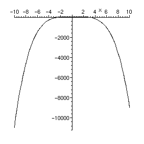
The plot command will draw our graph. It can take many options, but we just give it the name of our function,
which we have assigned to the variable poly, and a range for the x values . We are looking for the pieces

of the function which are bounded by the function above, and the x axis below. At first we try x from -10 to 10
to see how it looks.

> plot(poly, x= -10.. 10);

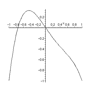
This doesn't show enough detail for what we want. We experiment by changing the range of x.
Using x between -1 and 1 will look good.

> plot(poly, x= -1 .. 1);

We see that the x values we want are approximately -.75 and 0.
We can do even better. fsolve will find all the roots of our funtion between any two given values.

> fsolve(poly, x = -1 .. .1);

The area we want will be the definite integral of our function between these values. We need to first
find the indefinite integral of our function. Here we'll be lazy and let the computer do the work.
The command int will compute the indefinite integral of a function. However, we should be able to do this
ourselves! We assign the area function to the variable f, so we can use it later.

> f := int (poly, x);

The same command int, will also compute the definite integral, which is the area we want. Here we
give it the lower and upper limits of integration which we computed above.

> int (poly, x = -.7548776662 .. 0);

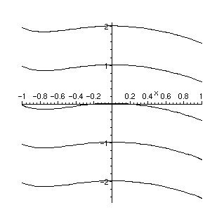
The general indefinite integral is a family of functions, differing from one another by constants. We give the
plot command a list of such functions, each differing by a constant.

> plot([f-2, f-1, f, f+1, f+2], x = -1 .. 1);

>